This example illustrates how you can iterate through an output database and search for the maximum value of von Mises stress. The script opens the output database specified by the first argument on the command line and iterates through the following:

• Each step.

• Each frame in each step.

• Each value of von Mises stress in each frame.

In addition, you can supply an optional assembly element set argument from the command line, in which case the script searches only the element set for the maximum value of von Mises stress.

The following illustrates how you can run the example script from the system prompt. The script will search the element set ALL ELEMENTS in the viewer tutorial output database for the maximum value of von Mises stress:

abaqus python odbMaxMises.py -odb viewer_tutorial.odb 
    -elset “ ALL ELEMENTS”

You can also run the example with only the -help parameter for a summary of the usage.

Use the following commands to retrieve the example script and the viewer tutorial output database:

abaqus fetch job=odbMaxMises.py
abaqus fetch job=viewer_tutorial

The following example illustrates how you can use the Abaqus Scripting Interface commands to do the following:

Use the following command to retrieve the example script:

abaqus fetch job=odbWrite

A FORTRAN program that reads the Abaqus results file and creates a deformed mesh from the original coordinate data and eigenvectors is described in “Creation of a perturbed mesh from original coordinate data and eigenvectors: FPERT,” Section 14.1.4 of the Abaqus Example Problems Manual. This example illustrates an Abaqus Scripting Interface script that reads an output database and performs similar calculations.

The command line arguments provide the following:

• odbName: The output database file name.

• modeList: A list of eigenmodes to use in the perturbation.

• weightList: The perturbation weighting factors.

• outNameUser: The output file name (optional).

Use the following command to retrieve the example script:

abaqus fetch job=odbPert

This example illustrates how you can operate on FieldOutput objects and save the computed field to the output database. The example script does the following:

• Retrieves two specified fields from the output database.

• Computes a new field by subtracting the fields that were retrieved.

• Creates a new Step object in the output database.

• Creates a new Frame object in the new step.

• Creates a new FieldOutput object in the new frame.

• Uses the addData method to add the computed field to the new FieldOutput object.

Use the following command to retrieve the example script:

abaqus fetch job=fieldOperation

The fetch command also retrieves an input file that you can use to generate the output database that is read by the example script.

This example illustrates how you can use the fieldValue operators to sum and average fieldValues in a region. The example script does the following:

• Retrieves the stress field for a specified region during the last step and frame of the output database.

• Sums all the stress fieldValues and computes the average value.

• For each component of stress, print the sum and the average stress.

Use the following command to retrieve the example script:

abaqus fetch job=sumRegionFieldValue

The fetch command also retrieves an input file that you can use to generate the output database that is read by the example script.

This example illustrates how you can use the historyOutput operators to compute the displacement magnitude from the components. The example script does the following:

• Retrieves the node of interest using a nodeSet.

• Uses the node of interest to construct a HistoryPoint object.

• Uses the HistoryPoint to retrieve the historyRegion.

• Computes the displacement magnitude history from the displacement component HistoryOutput objects in the historyRegion.

• Scales the displacement magnitude history using a predefined value.

• Prints the displacement magnitude history.

Use the following command to retrieve the example script:

abaqus fetch job=compDispMagHist

The fetch command also retrieves an input file that you can use to generate the output database that is read by the example script.

This example illustrates how you can use the frame operators to create a new load combination from existing load cases. The example script does the following:

• Retrieves the information describing the new load combination from the command line.

• Retrieves the frames for each load case.

• Computes the new stresses and displacements.

• Saves data computed to the output database as a new load combination.

The command line arguments provide the following:

• odbName: The output database file name.

• stepName: The name of the step containing the load cases.

• loadCaseNames: The load case names.

• scaling: The scale factors to apply to each load case.

Use the following command to retrieve the example script:

abaqus fetch job=createLoadComb

The fetch command also retrieves an input file that you can use to generate an output database that can be read by the example script.

This example illustrates how you can use the envelope operations to compute the stress range over a number of load cases. The example script does the following:

• For each load case during a specified step, the script collects the S11 components of the stress tensor fields into a list of scalar fields.

• Computes the maximum and minimum of the S11 stress component using the envelope calculations.

• Computes the stress range using the maximum and minimum values of the stress component.

• Creates a new frame in the step.

• Writes the computed stress range into a new FieldOutput object in the new frame.

Use the following command to retrieve the example script:

abaqus fetch job=stressRange

The fetch command also retrieves an input file that you can use to generate an output database that can be read by the example script.

This example illustrates how field results can be transformed to a different coordinate system. The example computes deviation of the nodal displacements with respect to a perfectly cylindrical displacement (cylinder bore distortion). The example does the following:

• Creates a cylindrical coordinate system.

• Transforms the results to the new coordinate system.

• Computes the average radial displacement.

• Computes the distortion as the difference between radial displacement and the average radial displacement.

• Saves the distortion field to the output database for viewing.

Use the following commands to retrieve the example script and an input file to create a sample output database:

abaqus fetch job=transformExa
abaqus fetch job=esf4sxdg

This example illustrates how you can view the results of a meshed beam cross-section analysis that was generated using Timoshenko beams, as described in “Meshed beam cross-sections,” Section 10.6 of the Abaqus Analysis User's Manual. Before you execute the example script, you must run two analyses that create the following output database files:

• An output database generated by the two-dimensional cross-section analysis. The script reads cross-section data, including the out-of-plane warping function, from this output database.

• An output database generated by the beam analysis. The script reads generalized section strains (SE) from this output database.

Use the following command to retrieve the example script:

abaqus fetch job=compositeBeam

You must run the script from Abaqus/CAE by selecting FileRun Script from the main menu bar. The script uses getInputs to display a dialog box that prompts you for the name of the output databases generated by the two-dimensional cross-section analysis and by the beam analysis. The names are case-insensitive, and you can omit the .odb file suffix. The files must be in the local directory. The dialog box also prompts you for the following:

• The name of the step

• The increment or mode number (for a frequency analysis)

• The name of the load case (if any)

• The name of the part instance

• The element number

• The integration point number

If you do not enter a value in a field, the script looks in the beam analysis output database for possible values. The script then enters a default value in the dialog box and displays information about the range of possible values in the Abaqus/CAE message area. You can leave the load case field blank if the analysis did not include load cases. The script does not continue until all the values in the dialog box are acceptable. The same values are written to a file called compositeBeam_values.dat in the local directory, and these values appear as defaults in the dialog box the next time you run the example script.

After the getInputs method returns acceptable values, the script reads the two output databases and writes the generated data back to the output database created by the two-dimensional cross-section analysis. The script then displays an undeformed contour plot of S11 and uses the getInputs method again to display a dialog box with a list of the available stress and strain components (S11, S22, S33, E11, E22, and E33). Click OK in this dialog box to cycle through the available components. Click Cancel to end the script. You can also select the component to display by starting the Visualization module and selecting ResultField Output from the main menu bar.

The example script writes new stress and strain fields. The script must provide a unique name for the generated field output because each of these fields is generated for a specific beam analysis output database and for a specific part instance, step, frame, element, and integration point. The script constructs this unique name as follows:

• All contour stress and strain fields for a specific beam analysis output database are written to a new frame, where the description of the frame is the name of the output database. For example, for a beam analysis output database called beam_run17.odb, the frame description is Beam ODB: beam_run17.

• The field name is assembled from a concatenation of the step name, frame index, instance name, element, and integration point, followed by E or S. For example, Step-1_4_LINEARMESHED_12_1_E. Any spaces in a step or instance name are replaced by underscores.

You can run the script many times; for example, to create contour data for a particular step, increment, and integration point along each element of the beam. In this case you would also use ResultField Output to select which element to display.

The contour data generated by the example script are written back to the output database that was originally created by the two-dimensional, cross-section analysis. If you want to preserve this database in its original form, you must save a copy before you run the example script.

This example illustrates how you can use the Abaqus Scripting Interface to compute acoustic far-field pressure values from infinite element sets and project the results onto a spherical surface for visualization purposes. The script extends the acoustic analysis functionality within Abaqus/Standard, as described in “Acoustic, shock, and coupled acoustic-structural analysis,” Section 6.10.1 of the Abaqus Analysis User's Manual, and “Infinite elements,” Section 28.3.1 of the Abaqus Analysis User's Manual. The script writes the acoustic far-field pressure values to an output database, and you can use Abaqus/CAE to view the far-field results.

The far-field pressure is defined as

where is the acoustic pressure at a distance from the reference point, is the wave number, and is the acoustic far-field pressure. The acoustic pressure decibel value is defined as where is the magnitude of the acoustic pressure at a point, is the root mean square acoustic pressure, and is the decibel reference value given as user input. The far-field pressure decibel value is defined in the same manner as , using the same reference value ().

The script also calculates the far-field acoustic intensity, which is defined as

where is the far-field rms pressure, is the fluid density, and c is the speed of sound in the medium.

Before you execute the script, you must run a direct-solution, steady-state dynamics acoustics analysis that includes three-dimensional acoustic infinite elements (ACIN3D3, ACIN3D4, ACIN3D6, and ACIN3D8). In addition, the output database must contain results for the following output variables:

• INFN, the acoustic infinite element normal vector.

• INFR, the acoustic infinite element “radius,” used in the coordinate map for these elements.

• PINF, the acoustic infinite element pressure coefficients.

Use the following command to retrieve the script:

abaqus fetch job=acousticVisualization 

Enter the Visualization module, and display the output database in the current viewport. Run the script by selecting FileRun Script from the main menu bar.

The script uses getInputs to display a dialog box that prompts you for the following information:

• The name of the element set containing the infinite elements (the name is case sensitive). By default, the script locates all the infinite elements in the model and uses them to create the spherical surface. If the script cannot find the specified element set in the output database, it displays a list of the available element sets in the message area.

• The radius of the sphere (required). The script asks you to enter a new value if the sphere with this radius does not intersect any of the selected infinite elements.

• The coordinates of the center of the sphere. By default, the script uses (0,0,0).

• The analysis steps. You can enter one of the following:

  • An Int

  • A comma-separated list of Ints

  • A range; for example, 1:20

  You can also enter a combination of Ints and ranges; for example, 4,5,10:20,30. By default, the script reads data from all the steps. The script ignores any steps that do not perform a direct-solution, steady-state dynamics acoustics analysis or that have no results.

• The frequencies for which output should be generated (Hz). You can enter a Float, a list of Floats, or a range. By default, the script generates output for all the frequencies in the original output database.

• A decibel reference value (required).

• The name of the part instance to create (required). The script appends this name to the name of the instance containing the infinite elements being used.

• The speed of sound (required).

• The fluid density (required)

• Whether to write data to the original output database. By default, the script writes to an output database called current-odb-name_acvis.odb.

After the getInputs method returns acceptable values, the script processes the elements in the specified element sets. The visualization sphere is then determined using the specified radius and center. For each element in the infinite element sets, the script creates a corresponding membrane element such that the new element is a projection of the old element onto the surface of the sphere. The projection uses the infinite element reference point and the internally calculated infinite direction normal (INFN) at each node of the element.

Once the new display elements have been created, the script writes results at the nodes in the set. The following output results are written back to the output database:

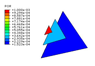
• POR, the acoustic pressure.

• PORdB, the acoustic pressure decibel value. If the reference value used is 2 × 10^–5 Pa, the PFARdB corresponds to dB SPL.

• PFAR, the acoustic far-field pressure.

• PFARdB, the far-field pressure decibel value.

• INTEN_FAR, the far-field acoustic intensity.

To create the output at each node, the script first determines the point at which the node ray intersects the sphere. Using the distance from the reference point to the intersection point and the element shape functions, the required output variables are calculated at the intersection point.

After the script has finished writing data, it opens the output database containing the new data. For comparison, the original instance is displayed along with the new instance, but results are available only for the new instance. However, if you chose to write the results back to the original output database, the original instance and the new instance along with the original results and the new results can be displayed side-by-side. The script displays any error, warning, or information messages in the message area.

You can run the script more than once and continue writing data to the same output database. For example, you can run the script several times to look at the far-field pressures at various points in space, and results on several spheres will be written to the output database.

To see how the script operates on a single triangular-element model, use the following command to retrieve the input file:

abaqus fetch job=singleTriangularElementModel

Use the following command to create the corresponding output database:

abaqus job=singleTriangularElementModel

The results from running the script twice using the single triangular-element model, changing the radius of the sphere, and writing the data back to the original output database are shown in Figure 9–6.

This model simulates the response of a sphere in “breathing” mode (a uniform radial expansion/compression mode). The model consists of one triangular ACIN3D3 element. Each node of the element is placed on a coordinate axis at a distance of 1.0 from the origin that serves as the reference point for the infinite element. The acoustic material properties do not have physical significance; the values used are for convenience only. The loading consists of applying an in-phase pressure boundary condition to all the nodes. Under this loading and geometry, the model behaves as a spherical source (an acoustic monopole) radiating in the radial direction only. The acoustic pressure, , and the acoustic far-field pressure, , at a distance from the center of the sphere are

and where is the known acoustic pressure at some reference distance and is the wave number.

For this single-element example, you should enter a value of 1.0 for the speed of sound; thus, , where is the frequency in Hz. in this model is 1, and is 0.001. The equations for the acoustic pressure, , and the acoustic far-field pressure, , reduce to

and

This example illustrates the use of an Abaqus Scripting Interface script to read selected element integration point records from an output database and to postprocess the elbow element results. The script creates X–Y data that can be plotted with the X–Y plotting capability in Abaqus/CAE. The script performs the same function as the FORTRAN program described in “Creation of a data file to facilitate the postprocessing of elbow element results: FELBOW,” Section 14.1.6 of the Abaqus Example Problems Manual.

The script reads integration point data for elbow elements from an output database to visualize one of the following:

The script creates either an ASCII file containing X–Y data or a new output database file that can be viewed using Abaqus/CAE.

To use option 2, you must ensure that the integration point coordinates (COORD) are written to the output database. For option 1 the X-data are data for the distance around the circumference of the elbow element, measured along the middle surface, and the Y-data are data for the output variable. For option 2 the X–Y data are the current coordinates of the middle-surface integration points around the circumference of the elbow element, projected to a local coordinate system in the plane of the deformed cross-section. The origin of the local system coincides with the center of the cross-section; the plane of the deformed cross-section is defined as the plane that contains the center of the cross-section.

You should specify the name of the output database during program execution. The script prompts for additional information, depending on the option that was chosen; this information includes the following:

• Your choice for storing results (ASCII file or a new output database)

• File name based on the above choice

• The postprocessing option (1 or 2)

• The part name

• The step name

• The frame number

• The element output variable (option 1 only)

• The component of the variable (option 1 only)

• The section point number (option 1 only)

• The element number or element set name

Before executing the script, run an analysis that creates an output database file containing the appropriate output. This analysis includes, for example, output for the elements and the integration point coordinates of the elements. Execute the script using the following command:

abaqus python felbow.py <filename.odb>

The script prompts for other information, such as the desired postprocessing option, part name, etc. The script processes the data and produces a text file or a new output database that contains the information required to visualize the elbow element results.

“Elastic-plastic collapse of a thin-walled elbow under in-plane bending and internal pressure,” Section 1.1.2 of the Abaqus Example Problems Manual, contains several figures that can be created with the aid of this program.