Products: Abaqus/Standard Abaqus/Explicit Abaqus/CAE
This section provides a reference to the axisymmetric solid elements available in Abaqus/Standard and Abaqus/Explicit.
Coordinate 1 is ![]() , coordinate 2 is
, coordinate 2 is ![]() . At
. At ![]() the r-direction corresponds to the global x-direction and the z-direction corresponds to the global y-direction. This is important when data must be given in global directions. Coordinate 1 must be greater than or equal to zero.
the r-direction corresponds to the global x-direction and the z-direction corresponds to the global y-direction. This is important when data must be given in global directions. Coordinate 1 must be greater than or equal to zero.
Degree of freedom 1 is ![]() , degree of freedom 2 is
, degree of freedom 2 is ![]() . Generalized axisymmetric elements with twist have an additional degree of freedom, 5, corresponding to the twist angle
. Generalized axisymmetric elements with twist have an additional degree of freedom, 5, corresponding to the twist angle ![]() (in radians).
(in radians).
Abaqus does not automatically apply any boundary conditions to nodes located along the symmetry axis. You must apply radial or symmetry boundary conditions on these nodes if desired.
In certain situations in Abaqus/Standard it may become necessary to apply radial boundary conditions on nodes that are located on the symmetry axis to obtain convergence in nonlinear problems. Therefore, the application of radial boundary conditions on nodes on the symmetry axis is recommended for nonlinear problems.
Point loads and moments, concentrated (nodal) fluxes, electrical currents, and seepage should be given as the value integrated around the circumference (that is, the total value on the ring).
| CAX3 | 3-node linear |
| CAX3H(S) | 3-node linear, hybrid with constant pressure |
| CAX4(S) | 4-node bilinear |
| CAX4H(S) | 4-node bilinear, hybrid with constant pressure |
| CAX4I(S) | 4-node bilinear, incompatible modes |
| CAX4IH(S) | 4-node bilinear, incompatible modes, hybrid with linear pressure |
| CAX4R | 4-node bilinear, reduced integration with hourglass control |
| CAX4RH(S) | 4-node bilinear, reduced integration with hourglass control, hybrid with constant pressure |
| CAX6(S) | 6-node quadratic |
| CAX6H(S) | 6-node quadratic, hybrid with linear pressure |
| CAX6M | 6-node modified, with hourglass control |
| CAX6MH(S) | 6-node modified, with hourglass control, hybrid with linear pressure |
| CAX8(S) | 8-node biquadratic |
| CAX8H(S) | 8-node biquadratic, hybrid with linear pressure |
| CAX8R(S) | 8-node biquadratic, reduced integration |
| CAX8RH(S) | 8-node biquadratic, reduced integration, hybrid with linear pressure |
The constant pressure hybrid elements have one additional variable and the linear pressure elements have three additional variables relating to pressure.
Element types CAX4I and CAX4IH have five additional variables relating to the incompatible modes.
Element types CAX6M and CAX6MH have two additional displacement variables.
| CGAX3(S) | 3-node linear |
| CGAX3H(S) | 3-node linear, hybrid with constant pressure |
| CGAX4(S) | 4-node bilinear |
| CGAX4H(S) | 4-node bilinear, hybrid with constant pressure |
| CGAX4R(S) | 4-node bilinear, reduced integration with hourglass control |
| CGAX4RH(S) | 4-node bilinear, reduced integration with hourglass control, hybrid with constant pressure |
| CGAX6(S) | 6-node quadratic |
| CGAX6H(S) | 6-node quadratic, hybrid with linear pressure |
| CGAX6M(S) | 6-node modified, with hourglass control |
| CGAX6MH(S) | 6-node modified, with hourglass control, hybrid with linear pressure |
| CGAX8(S) | 8-node biquadratic |
| CGAX8H(S) | 8-node biquadratic, hybrid with linear pressure |
| CGAX8R(S) | 8-node biquadratic, reduced integration |
| CGAX8RH(S) | 8-node biquadratic, reduced integration, hybrid with linear pressure |
| DCAX3(S) | 3-node linear |
| DCAX4(S) | 4-node linear |
| DCAX6(S) | 6-node quadratic |
| DCAX8(S) | 8-node quadratic |
| DCCAX2(S) | 2-node |
| DCCAX2D(S) | 2-node with dispersion control |
| DCCAX4(S) | 4-node |
| DCCAX4D(S) | 4-node with dispersion control |
| DCAX3E(S) | 3-node linear |
| DCAX4E(S) | 4-node linear |
| DCAX6E(S) | 6-node quadratic |
| DCAX8E(S) | 8-node quadratic |
| CAX3T | 3-node linear displacement and temperature |
| CAX4T(S) | 4-node bilinear displacement and temperature |
| CAX4HT(S) | 4-node bilinear displacement and temperature, hybrid with constant pressure |
| CAX4RT | 4-node bilinear displacement and temperature, reduced integration with hourglass control |
| CAX4RHT(S) | 4-node bilinear displacement and temperature, reduced integration with hourglass control, hybrid with constant pressure |
| CAX6MT | 6-node modified displacement and temperature, with hourglass control |
| CAX6MHT(S) | 6-node modified displacement and temperature, with hourglass control, hybrid with linear pressure |
| CAX8T(S) | 8-node biquadratic displacement, bilinear temperature |
| CAX8HT(S) | 8-node biquadratic displacement, bilinear temperature, hybrid with linear pressure |
| CAX8RT(S) | 8-node biquadratic displacement, bilinear temperature, reduced integration |
| CAX8RHT(S) | 8-node biquadratic displacement, bilinear temperature, reduced integration, hybrid with linear pressure |
| CGAX3T(S) | 3-node linear displacement and temperature |
| CGAX3HT(S) | 3-node linear displacement and temperature, hybrid with constant pressure |
| CGAX4T(S) | 4-node bilinear displacement and temperature |
| CGAX4HT(S) | 4-node bilinear displacement and temperature, hybrid with constant pressure |
| CGAX4RT(S) | 4-node bilinear displacement and temperature, reduced integration with hourglass control |
| CGAX4RHT(S) | 4-node bilinear displacement and temperature, reduced integration with hourglass control, hybrid with constant pressure |
| CGAX6MT(S) | 6-node modified displacement and temperature, with hourglass control |
| CGAX6MHT(S) | 6-node modified displacement and temperature, with hourglass control, hybrid with constant pressure |
| CGAX8T(S) | 8-node biquadratic displacement, bilinear temperature |
| CGAX8HT(S) | 8-node biquadratic displacement, bilinear temperature, hybrid with linear pressure |
| CGAX8RT(S) | 8-node biquadratic displacement, bilinear temperature, reduced integration |
| CGAX8RHT(S) | 8-node biquadratic displacement, bilinear temperature, reduced integration, hybrid with linear pressure |
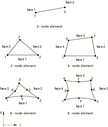
1, 2, 5, 11 at corner nodes
1, 2, 5 at midside nodes of second-order elements
1, 2, 5, 11 at midside nodes of the modified displacement and temperature elements
The constant pressure hybrid elements have one additional variable and the linear pressure elements have three additional variables relating to pressure.
Element types CGAX6MT and CGAX6MHT have two additional displacement variables and one additional temperature variable.
| CAX4P(S) | 4-node bilinear displacement and pore pressure |
| CAX4PH(S) | 4-node bilinear displacement and pore pressure, hybrid with constant pressure |
| CAX4RP(S) | 4-node bilinear displacement and pore pressure, reduced integration with hourglass control |
| CAX4RPH(S) | 4-node bilinear displacement and pore pressure, reduced integration with hourglass control, hybrid with constant pressure |
| CAX6MP(S) | 6-node modified displacement and pore pressure, with hourglass control |
| CAX6MPH(S) | 6-node modified displacement and pore pressure, with hourglass control, hybrid with linear pressure |
| CAX8P(S) | 8-node biquadratic displacement, bilinear pore pressure |
| CAX8PH(S) | 8-node biquadratic displacement, bilinear pore pressure, hybrid with linear pressure |
| CAX8RP(S) | 8-node biquadratic displacement, bilinear pore pressure, reduced integration |
| CAX8RPH(S) | 8-node biquadratic displacement, bilinear pore pressure, reduced integration, hybrid with linear pressure |
The constant pressure hybrid elements have one additional variable relating to the effective pressure stress, and the linear pressure hybrid elements have three additional variables relating to the effective pressure stress to permit fully incompressible material modeling.
Element types CAX6MP and CAX6MPH have two additional displacement variables and one additional pore pressure variable.
| CAX4PT(S) | 4-node bilinear displacement, pore pressure, and temperature |
| CAX4RPT(S) | 4-node bilinear displacement, pore pressure, and temperature; reduced integration with hourglass control |
| CAX4RPHT(S) | 4-node bilinear displacement, pore pressure, and temperature; reduced integration with hourglass control, hybrid with constant pressure |
For element types DCCAX2 and DCCAX2D, you must specify the channel thickness of the element in the (r–z) plane. The default is unit thickness if no thickness is given.
For all other elements, you do not need to specify the thickness.
| Input File Usage: | *SOLID SECTION |
| Abaqus/CAE Usage: | Property module: Create Section: select Solid as the section Category and Homogeneous as the section Type |
Distributed loads are available for all elements with displacement degrees of freedom. They are specified as described in “Distributed loads,” Section 33.4.3. Distributed load magnitudes are per unit area or per unit volume. They do not need to be multiplied by ![]() .
.
Load ID (*DLOAD): BR
Abaqus/CAE Load/Interaction: Body force
Units: FL3
Description: Body force in radial direction.
Load ID (*DLOAD): BZ
Abaqus/CAE Load/Interaction: Body force
Units: FL3
Description: Body force in axial direction.
Load ID (*DLOAD): BRNU
Abaqus/CAE Load/Interaction: Body force
Units: FL3
Description: Nonuniform body force in radial direction with magnitude supplied via user subroutine DLOAD in Abaqus/Standard and VDLOAD in Abaqus/Explicit.
Load ID (*DLOAD): BZNU
Abaqus/CAE Load/Interaction: Body force
Units: FL3
Description: Nonuniform body force in axial direction with magnitude supplied via user subroutine DLOAD in Abaqus/Standard and VDLOAD in Abaqus/Explicit.
Load ID (*DLOAD): CENT(S)
Abaqus/CAE Load/Interaction: Not supported
Units: FL4M3T2
Description: Centrifugal load (magnitude input as ![]() , where
, where ![]() is the mass density per unit volume,
is the mass density per unit volume, ![]() is the angular velocity). Not available for pore pressure elements.
is the angular velocity). Not available for pore pressure elements.
Load ID (*DLOAD): CENTRIF(S)
Abaqus/CAE Load/Interaction: Rotational body force
Units: T2
Description: Centrifugal load (magnitude is input as ![]() , where
, where ![]() is the angular velocity).
is the angular velocity).
Load ID (*DLOAD): GRAV
Abaqus/CAE Load/Interaction: Gravity
Units: LT2
Description: Gravity loading in a specified direction (magnitude is input as acceleration).
Load ID (*DLOAD): HPn(S)
Abaqus/CAE Load/Interaction: Not supported
Units: FL2
Description: Hydrostatic pressure on face n, linear in global Y.
Load ID (*DLOAD): Pn
Abaqus/CAE Load/Interaction: Pressure
Units: FL2
Description: Pressure on face n.
Load ID (*DLOAD): PnNU
Abaqus/CAE Load/Interaction: Not supported
Units: FL2
Description: Nonuniform pressure on face n with magnitude supplied via user subroutine DLOAD in Abaqus/Standard and VDLOAD in Abaqus/Explicit.
Load ID (*DLOAD): SBF(E)
Abaqus/CAE Load/Interaction: Not supported
Units: FL5T2
Description: Stagnation body force in radial and axial directions.
Load ID (*DLOAD): SPn(E)
Abaqus/CAE Load/Interaction: Not supported
Units: FL4T2
Description: Stagnation pressure on face n.
Load ID (*DLOAD): TRSHRn
Abaqus/CAE Load/Interaction: Surface traction
Units: FL2
Description: Shear traction on face n.
Load ID (*DLOAD): TRSHRnNU(S)
Abaqus/CAE Load/Interaction: Not supported
Units: FL2
Description: Nonuniform shear traction on face n with magnitude and direction supplied via user subroutine UTRACLOAD.
Load ID (*DLOAD): TRVECn
Abaqus/CAE Load/Interaction: Surface traction
Units: FL2
Description: General traction on face n.
Load ID (*DLOAD): TRVECnNU(S)
Abaqus/CAE Load/Interaction: Not supported
Units: FL2
Description: Nonuniform general traction on face n with magnitude and direction supplied via user subroutine UTRACLOAD.
Load ID (*DLOAD): VBF(E)
Abaqus/CAE Load/Interaction: Not supported
Units: FL4T
Description: Viscous body force in radial and axial directions.
Load ID (*DLOAD): VPn(E)
Abaqus/CAE Load/Interaction: Not supported
Units: FL3T
Description: Viscous pressure on face n, applying a pressure proportional to the velocity normal to the face and opposing the motion.
Foundations are available for Abaqus/Standard elements with displacement degrees of freedom. They are specified as described in “Element foundations,” Section 2.2.2.
Load ID (*FOUNDATION): Fn(S)
Abaqus/CAE Load/Interaction: Elastic foundation
Units: FL3
Description: Elastic foundation on face n. For CGAX elements the elastic foundations are applied to degrees of freedom ![]() and
and ![]() only.
only.
Distributed heat fluxes are available for all elements with temperature degrees of freedom. They are specified as described in “Thermal loads,” Section 33.4.4. Distributed heat flux magnitudes are per unit area or per unit volume. They do not need to be multiplied by ![]() .
.
Load ID (*DFLUX): BF
Abaqus/CAE Load/Interaction: Body heat flux
Units: JL3T1
Description: Heat body flux per unit volume.
Load ID (*DFLUX): BFNU(S)
Abaqus/CAE Load/Interaction: Body heat flux
Units: JL3T1
Description: Nonuniform heat body flux per unit volume with magnitude supplied via user subroutine DFLUX.
Load ID (*DFLUX): Sn
Abaqus/CAE Load/Interaction: Surface heat flux
Units: JL2T1
Description: Heat surface flux per unit area into face n.
Load ID (*DFLUX): SnNU(S)
Abaqus/CAE Load/Interaction: Not supported
Units: JL2T1
Description: Nonuniform heat surface flux per unit area into face n with magnitude supplied via user subroutine DFLUX.
Film conditions are available for all elements with temperature degrees of freedom. They are specified as described in “Thermal loads,” Section 33.4.4.
Load ID (*FILM): Fn
Abaqus/CAE Load/Interaction: Surface film condition
Units: JL2T1![]() 1
1
Description: Film coefficient and sink temperature (units of ![]() ) provided on face n.
) provided on face n.
Load ID (*FILM): FnNU(S)
Abaqus/CAE Load/Interaction: Not supported
Units: JL2T1![]() 1
1
Description: Nonuniform film coefficient and sink temperature (units of ![]() ) provided on face n with magnitude supplied via user subroutine FILM.
) provided on face n with magnitude supplied via user subroutine FILM.
Radiation conditions are available for all elements with temperature degrees of freedom. They are specified as described in “Thermal loads,” Section 33.4.4.
Load ID (*RADIATE): Rn
Abaqus/CAE Load/Interaction: Surface radiation
Units: Dimensionless
Description: Emissivity and sink temperature provided for face n.
Distributed flows are available for all elements with pore pressure degrees of freedom. They are specified as described in “Pore fluid flow,” Section 33.4.7. Distributed flow magnitudes are per unit area or per unit volume. They do not need to be multiplied by ![]() .
.
Load ID (*FLOW): Qn(S)
Abaqus/CAE Load/Interaction: Not supported
Units: F1L3T1
Description: Seepage coefficient and reference sink pore pressure (units of FL2) provided on face n.
Load ID (*FLOW): QnD(S)
Abaqus/CAE Load/Interaction: Not supported
Units: F1L3T1
Description: Drainage-only seepage coefficient provided on face n.
Load ID (*FLOW): QnNU(S)
Abaqus/CAE Load/Interaction: Not supported
Units: F1L3T1
Description: Nonuniform seepage coefficient and reference sink pore pressure (units of FL2) provided on face n with magnitude supplied via user subroutine FLOW.
Load ID (*DFLOW): Sn(S)
Abaqus/CAE Load/Interaction: Surface pore fluid
Units: LT1
Description: Prescribed pore fluid effective velocity (outward from the face) on face n.
Load ID (*DFLOW): SnNU(S)
Abaqus/CAE Load/Interaction: Not supported
Units: LT1
Description: Nonuniform prescribed pore fluid effective velocity (outward from the face) on face n with magnitude supplied via user subroutine DFLOW.
Distributed impedances are available for all elements with acoustic pressure degrees of freedom. They are specified as described in “Acoustic and shock loads,” Section 33.4.6.
Load ID (*IMPEDANCE): In
Abaqus/CAE Load/Interaction: Not supported
Units: None
Description: Name of the impedance property that defines the impedance on face n.
Electric fluxes are available for piezoelectric elements. They are specified as described in “Piezoelectric analysis,” Section 6.7.2.
Load ID (*DECHARGE): EBF(S)
Abaqus/CAE Load/Interaction: Body charge
Units: CL3
Description: Body flux per unit volume.
Load ID (*DECHARGE): ESn(S)
Abaqus/CAE Load/Interaction: Surface charge
Units: CL2
Description: Prescribed surface charge on face n.
Distributed electric current densities are available for coupled thermal-electrical elements. They are specified as described in “Coupled thermal-electrical analysis,” Section 6.7.3.
Load ID (*DECURRENT): CBF(S)
Abaqus/CAE Load/Interaction: Body current
Units: CL3T1
Description: Volumetric current source density.
Load ID (*DECURRENT): CSn(S)
Abaqus/CAE Load/Interaction: Surface current
Units: CL2T1
Description: Current density on face n.
Distributed concentration fluxes are available for mass diffusion elements. They are specified as described in “Mass diffusion analysis,” Section 6.9.1.
Load ID (*DFLUX): BF(S)
Abaqus/CAE Load/Interaction: Body concentration flux
Units: PT1
Description: Concentration body flux per unit volume.
Load ID (*DFLUX): BFNU(S)
Abaqus/CAE Load/Interaction: Body concentration flux
Units: PT1
Description: Nonuniform concentration body flux per unit volume with magnitude supplied via user subroutine DFLUX.
Load ID (*DFLUX): Sn(S)
Abaqus/CAE Load/Interaction: Surface concentration flux
Units: PLT1
Description: Concentration surface flux per unit area into face n.
Load ID (*DFLUX): SnNU(S)
Abaqus/CAE Load/Interaction: Surface concentration flux
Units: PLT1
Description: Nonuniform concentration surface flux per unit area into face n with magnitude supplied via user subroutine DFLUX.
Surface-based distributed loads are available for all elements with displacement degrees of freedom. They are specified as described in “Distributed loads,” Section 33.4.3. Distributed load magnitudes are per unit area or per unit volume. They do not need to be multiplied by ![]() .
.
Load ID (*DSLOAD): HP(S)
Abaqus/CAE Load/Interaction: Pressure
Units: FL2
Description: Hydrostatic pressure on the element surface, linear in global Y.
Load ID (*DSLOAD): P
Abaqus/CAE Load/Interaction: Pressure
Units: FL2
Description: Pressure on the element surface.
Load ID (*DSLOAD): PNU
Abaqus/CAE Load/Interaction: Pressure
Units: FL2
Description: Nonuniform pressure on the element surface with magnitude supplied via user subroutine DLOAD in Abaqus/Standard and VDLOAD in Abaqus/Explicit.
Load ID (*DSLOAD): SP(E)
Abaqus/CAE Load/Interaction: Pressure
Units: FL4T2
Description: Stagnation pressure on the element surface.
Load ID (*DSLOAD): TRSHR
Abaqus/CAE Load/Interaction: Surface traction
Units: FL2
Description: Shear traction on the element surface.
Load ID (*DSLOAD): TRSHRNU(S)
Abaqus/CAE Load/Interaction: Surface traction
Units: FL2
Description: Nonuniform shear traction on the element surface with magnitude and direction supplied via user subroutine UTRACLOAD.
Load ID (*DSLOAD): TRVEC
Abaqus/CAE Load/Interaction: Surface traction
Units: FL2
Description: General traction on the element surface.
Load ID (*DSLOAD): TRVECNU(S)
Abaqus/CAE Load/Interaction: Surface traction
Units: FL2
Description: Nonuniform general traction on the element surface with magnitude and direction supplied via user subroutine UTRACLOAD.
Load ID (*DSLOAD): VP(E)
Abaqus/CAE Load/Interaction: Pressure
Units: FL3T
Description: Viscous pressure applied on the element surface. The viscous pressure is proportional to the velocity normal to the face and opposing the motion.
Surface-based heat fluxes are available for all elements with temperature degrees of freedom. They are specified as described in “Thermal loads,” Section 33.4.4. Distributed heat flux magnitudes are per unit area or per unit volume. They do not need to be multiplied by ![]() .
.
Load ID (*DSFLUX): S
Abaqus/CAE Load/Interaction: Surface heat flux
Units: JL2T1
Description: Heat surface flux per unit area into the element surface.
Load ID (*DSFLUX): SNU(S)
Abaqus/CAE Load/Interaction: Surface heat flux
Units: JL2T1
Description: Nonuniform heat surface flux per unit area into the element surface with magnitude supplied via user subroutine DFLUX.
Surface-based film conditions are available for all elements with temperature degrees of freedom. They are specified as described in “Thermal loads,” Section 33.4.4.
Load ID (*SFILM): F
Abaqus/CAE Load/Interaction: Surface film condition
Units: JL2T1![]() 1
1
Description: Film coefficient and sink temperature (units of ![]() ) provided on the element surface.
) provided on the element surface.
Load ID (*SFILM): FNU(S)
Abaqus/CAE Load/Interaction: Surface film condition
Units: JL2T1![]() 1
1
Description: Nonuniform film coefficient and sink temperature (units of ![]() ) provided on the element surface with magnitude supplied via user subroutine FILM.
) provided on the element surface with magnitude supplied via user subroutine FILM.
Surface-based radiation conditions are available for all elements with temperature degrees of freedom. They are specified as described in “Thermal loads,” Section 33.4.4.
Load ID (*SRADIATE): R
Abaqus/CAE Load/Interaction: Surface radiation
Units: Dimensionless
Description: Emissivity and sink temperature provided for the element surface.
Surface-based distributed flows are available for all elements with pore pressure degrees of freedom. They are specified as described in “Pore fluid flow,” Section 33.4.7. Distributed flow magnitudes are per unit area or per unit volume. They do not need to be multiplied by ![]() .
.
Load ID (*SFLOW): Q(S)
Abaqus/CAE Load/Interaction: Not supported
Units: F1L3T1
Description: Seepage coefficient and reference sink pore pressure (units of FL2) provided on the element surface.
Load ID (*SFLOW): QD(S)
Abaqus/CAE Load/Interaction: Not supported
Units: F1L3T1
Description: Drainage-only seepage coefficient provided on the element surface.
Load ID (*SFLOW): QNU(S)
Abaqus/CAE Load/Interaction: Not supported
Units: F1L3T1
Description: Nonuniform seepage coefficient and reference sink pore pressure (units of FL2) provided on the element surface with magnitude supplied via user subroutine FLOW.
Load ID (*DSFLOW): S(S)
Abaqus/CAE Load/Interaction: Surface pore fluid
Units: LT1
Description: Prescribed pore fluid effective velocity outward from the element surface.
Load ID (*DSFLOW): SNU(S)
Abaqus/CAE Load/Interaction: Surface pore fluid
Units: LT1
Description: Nonuniform prescribed pore fluid effective velocity outward from the element surface with magnitude supplied via user subroutine DFLOW.
Surface-based impedances are available for all elements with acoustic pressure degrees of freedom. They are specified as described in “Acoustic and shock loads,” Section 33.4.6.
Surface-based incident wave loads are available for all elements with displacement degrees of freedom or acoustic pressure degrees of freedom. They are specified as described in “Acoustic and shock loads,” Section 33.4.6. If the incident wave field includes a reflection off a plane outside the boundaries of the mesh, this effect can be included.
Surface-based electric fluxes are available for piezoelectric elements. They are specified as described in “Piezoelectric analysis,” Section 6.7.2.
Load ID (*DSECHARGE): ES(S)
Abaqus/CAE Load/Interaction: Surface charge
Units: CL2
Description: Prescribed surface charge on the element surface.
Surface-based electric current densities are available for coupled thermal-electrical elements. They are specified as described in “Coupled thermal-electrical analysis,” Section 6.7.3.
Load ID (*DSECURRENT): CS(S)
Abaqus/CAE Load/Interaction: Surface current
Units: CL2T1
Description: Current density on the element surface.
Output is in global directions unless a local coordinate system is assigned to the element through the section definition (“Orientations,” Section 2.2.5) in which case output is in the local coordinate system (which rotates with the motion in large-displacement analysis). See “State storage,” Section 1.5.4 of the Abaqus Theory Manual, for details. For regular axisymmetric elements, the local orientation must be in the ![]() –z plane with
–z plane with ![]() being a principal direction. For generalized axisymmetric elements with twist, the local orientation can be arbitrary.
being a principal direction. For generalized axisymmetric elements with twist, the local orientation can be arbitrary.
Stress and other tensors (including strain tensors) are available for elements with displacement degrees of freedom. All tensors have the same components. For example, the stress components are as follows:
S11 | Stress in the radial direction or in the local 1-direction. |
S22 | Stress in the axial direction or in the local 2-direction. |
S33 | Hoop direct stress. |
S12 | Shear stress. |
S11 | Stress in the radial direction or in the local 1-direction. |
S22 | Stress in the axial direction or in the local 2-direction. |
S33 | Stress in the circumferential direction or in the local 3-direction. |
S12 | Shear stress. |
S13 | Shear stress. |
S23 | Shear stress. |
Available for elements with temperature degrees of freedom.
HFL1 | Heat flux in the radial direction or in the local 1-direction. |
HFL2 | Heat flux in the axial direction or in the local 2-direction. |
Available for elements with pore pressure degrees of freedom, except for acoustic elements.
FLVEL1 | Pore fluid effective velocity in the radial direction or in the local 1-direction. |
FLVEL2 | Pore fluid effective velocity in the axial direction or in the local 2-direction. |
Available for elements with normalized concentration degrees of freedom.
MFL1 | Concentration flux in the radial direction or in the local 1-direction. |
MFL2 | Concentration flux in the axial direction or in the local 2-direction. |
Available for elements with electrical potential degrees of freedom.
EPG1 | Electrical potential gradient in the 1-direction. |
EPG2 | Electrical potential gradient in the 2-direction. |
For heat transfer applications a different integration scheme is used for triangular elements, as described in “Triangular, tetrahedral, and wedge elements,” Section 3.2.6 of the Abaqus Theory Manual.