Product: Abaqus/Explicit
Connector uniaxial behavior:
can be defined in any connector with available components of relative motion by specifying the loading and unloading behavior;
can be specified for each available component of relative motion independently;
can define separate response in the tensile and compressive directions;
can exhibit nonlinear elastic behavior, damaged elastic behavior, or elastic-plastic type behavior with permanent deformation upon complete unloading;
can have an unloading response specified; and
can be specified as dependent on constitutive motions in several local directions.
The local directions for each connection type (as described in “Connection-type library,” Section 31.1.5) determine the directions in which the forces and moments act and in which the displacements and rotations are measured.
Uniaxial behavior can be specified for an available component of relative motion by defining the loading and unloading response for that component. For each component, separate loading/unloading response data can be defined for the response in the tensile and compressive directions. The loading and unloading response can be classified according to three available behavior types:
nonlinear elastic behavior;
damaged elastic behavior; and
elastic-plastic type behavior with permanent deformation.
To define the loading response, you specify forces or moments as nonlinear functions of the components of relative motion. These functions can also depend on temperature, field variables, and constitutive displacements/rotations in the other component directions. See “Input syntax rules,” Section 1.2.1, for further information about defining data as functions of temperature and field variables.
The unloading response can be defined in the following ways:
You can specify several unloading curves that express the forces or moments as nonlinear functions of the components of relative motion; Abaqus interpolates these curves to create an unloading curve that passes through the point of unloading in an analysis.
You can specify an energy dissipation factor (and a permanent deformation factor for models with permanent deformation), from which Abaqus calculates an exponential/quadratic unloading function.
You can specify the forces or moments as nonlinear functions of the components of relative motion, as well as a transition slope; the connector unloads along the specified transition slope until it intersects the specified unloading function, at which point it unloads according to the function. (This unloading definition is referred to as combined unloading.)
You can specify the forces or moments as nonlinear functions of the components of relative motion; Abaqus shifts the specified unloading function along the strain axis so that it passes through the point of unloading in an analysis.
Table 31.2.10–1 Available unloading definitions for the uniaxial behavior types.
| Material behavior type | Unloading definition | ||||
|---|---|---|---|---|---|
| Interpolated | Quadratic | Exponential | Combined | Shifted | |
| Rate-dependent elastic | |||||
| Damaged elastic | |||||
| Permanent deformation | |||||
| Input File Usage: | Use the following options to define connector uniaxial behavior: |
*CONNECTOR BEHAVIOR, NAME=name *CONNECTOR UNIAXIAL BEHAVIOR, COMPONENT=component number *LOADING DATA, DIRECTION=deformation direction, TYPE=behavior type data lines to define loading data *UNLOADING DATA data lines to define unloading data |
The loading/unloading data can be defined separately for tension and compression by specifying the deformation direction. If the deformation direction is defined (tension or compression), the tabular values defining tensile or compressive behavior should be specified with positive values of forces/moments and displacements/rotations in the specified component of relative motion and the loading data must start at the origin. If the behavior is not defined in a loading direction, the force response will be zero in that direction (the connector has no resistance in that direction).
If the deformation direction is not defined, the data apply to both tension and compression. However, the behavior is then considered to be nonlinear elastic and no damage or permanent deformation can be specified. The response data will be considered to be symmetric about the origin if either tensile or compressive data are omitted.
| Input File Usage: | Use the following option to define tensile behavior: |
*LOADING DATA, DIRECTION=TENSION Use the following option to define compressive behavior: *LOADING DATA, DIRECTION=COMPRESSION Use the following option to define both tensile compressive behavior in a single table: *LOADING DATA |
By default, the loading and unloading functions depend only on the displacement or rotation in the direction of the component of relative motion specified for the connector uniaxial behavior definition (see “Connector behavior,” Section 31.2.1, for details). However, it is also possible to define loading and unloading functions that depend on the constitutive displacements and rotations in multiple component directions.
| Input File Usage: | Use the following option to define connector uniaxial behavior that depends on the relative displacements and/or rotations in several component directions: |
*LOADING DATA, INDEPENDENT COMPONENTS=CONSTITUTIVE MOTION |
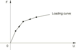
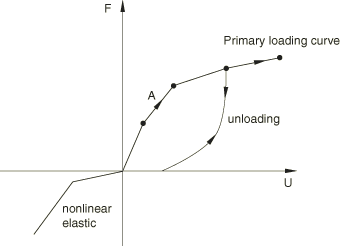
When the loading response is rate independent, the unloading response is also rate independent and occurs along the same user-specified loading curve as illustrated in Figure 31.2.10–1. An unloading curve does not need to be specified.
| Input File Usage: | *LOADING DATA, TYPE=ELASTIC |
The rate-dependent models require the specification of force-displacement curves at different rates of deformation to describe both loading and unloading behavior. If unloading behavior is not specified, the unloading occurs along the loading curve with the smallest rate of deformation. As the rate of deformation changes, the response is obtained by interpolation of the specified loading/unloading data. Unphysical jumps in the forces due to sudden changes in the rate of deformation are prevented using a technique based on viscoplastic regularization. This technique also helps model relaxation effects in a very simplistic manner, with the relaxation time given as ![]() where
where ![]() ,
, ![]() , and
, and ![]() are material parameters and
are material parameters and ![]() is the stretch.
is the stretch. ![]() is a linear viscosity parameter that controls the relaxation time when
is a linear viscosity parameter that controls the relaxation time when ![]() . Small values of this parameter should be used.
. Small values of this parameter should be used. ![]() is a nonlinear viscosity parameter that controls the relaxation time at higher values of
is a nonlinear viscosity parameter that controls the relaxation time at higher values of ![]() . The smaller this value, the shorter the relaxation time.
. The smaller this value, the shorter the relaxation time. ![]() controls the sensitivity of the relaxation speed to the stretch in the component of relative motion. Suggested values of these parameters are
controls the sensitivity of the relaxation speed to the stretch in the component of relative motion. Suggested values of these parameters are ![]() ,
, ![]() , and
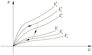
, and ![]() . Figure 31.2.10–2 illustrates the loading/unloading behavior as the connector is loaded at a rate
. Figure 31.2.10–2 illustrates the loading/unloading behavior as the connector is loaded at a rate ![]() and then unloaded at a rate
and then unloaded at a rate ![]() .
.
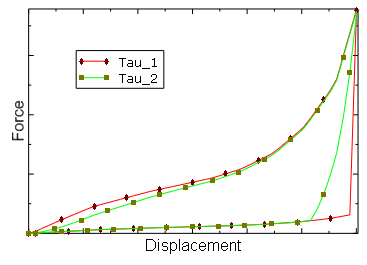
Figure 31.2.10–3 shows the loading/unloading response of a connector element for two different relaxation times ![]() and
and ![]() with
with ![]() . The larger the relaxation time, the longer it takes to achieve the specified loading/unloading response for the applied deformation rate.
. The larger the relaxation time, the longer it takes to achieve the specified loading/unloading response for the applied deformation rate.
| Input File Usage: | Use the following options when the unloading is also rate dependent: |
*LOADING DATA, TYPE=ELASTIC, RATE DEPENDENT
*UNLOADING DATA, DEFINITION=INTERPOLATED CURVE,
RATE DEPENDENT
Use the following options when the unloading is rate independent: *LOADING DATA, TYPE=ELASTIC, RATE DEPENDENT *UNLOADING DATA, DEFINITION=INTERPOLATED CURVE |
The damage models dissipate energy upon unloading, and there is no permanent deformation upon complete unloading. The unloading behavior controls the amount of energy dissipated by damage mechanisms and can be specified in one of the following ways:
an analytical unloading curve (exponential/quadratic);
an unloading curve interpolated from multiple user-specified unloading curves; or
unloading along a transition unloading curve (constant slope specified by user) to the user-specified unloading curve (combined unloading).
You can specify the onset of damage by defining the displacement below which unloading occurs along the loading curve.
| Input File Usage: | *LOADING DATA, TYPE=DAMAGE, DAMAGE ONSET=value |
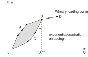
The damage model in Figure 31.2.10–4 is based on an analytical unloading curve that is derived from an energy dissipation factor, ![]() (fraction of energy that is dissipated at any displacement level). As the connector is loaded, the force follows the path given by the loading curve. If the connector is unloaded (for example, at point B), the force follows the unloading curve
(fraction of energy that is dissipated at any displacement level). As the connector is loaded, the force follows the path given by the loading curve. If the connector is unloaded (for example, at point B), the force follows the unloading curve ![]() . Reloading after unloading follows the unloading curve
. Reloading after unloading follows the unloading curve ![]() until the loading is such that the displacement becomes greater than
until the loading is such that the displacement becomes greater than ![]() , after which the loading path follows the loading curve. The arrows shown in Figure 31.2.10–4 illustrate the loading/unloading paths of this model.
, after which the loading path follows the loading curve. The arrows shown in Figure 31.2.10–4 illustrate the loading/unloading paths of this model.
The unloading response follows the loading curve when the calculated unloading curve lies above the loading curve to prevent energy generation and follows a zero force response when the unloading curve yields a negative response. In such cases the dissipated energy will be less than the value specified by the energy dissipation factor.
| Input File Usage: | Use the following option to define quadratic unloading behavior: |
*UNLOADING DATA, DEFINITION=QUADRATIC Use the following option to define exponential unloading behavior: *UNLOADING DATA, DEFINITION=EXPONENTIAL |
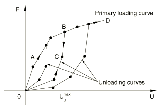
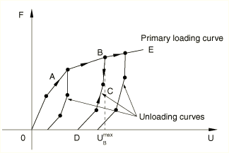
The damage model in Figure 31.2.10–5 illustrates an interpolated unloading response based on multiple unloading curves that intersect the primary loading curve at increasing values of forces/displacements. You can specify as many unloading curves as are necessary to define the unloading response. Each unloading curve always starts at point O, the point of zero force and zero displacements, since the damage models do not allow any permanent deformation. The unloading curves are stored in normalized form so that they intersect the loading curve at a unit force for a unit displacement, and the interpolation occurs between these normalized curves. If unloading occurs from a maximum displacement for which an unloading curve is not specified, the unloading is interpolated from neighboring unloading curves. As the connector is loaded, the force follows the path given by the loading curve. If the connector is unloaded (for example, at point B), the force follows the unloading curve ![]() . Reloading after unloading follows the unloading path
. Reloading after unloading follows the unloading path ![]() until the loading is such that the displacement becomes greater than
until the loading is such that the displacement becomes greater than ![]() , after which the loading path follows the loading curve.
, after which the loading path follows the loading curve.
If the loading curve depends on the constitutive displacements/rotations in several component directions, the unloading curves also depend on the same component directions. The unloading curves also have the same temperature and field variable dependencies as the loading curve.
| Input File Usage: | *UNLOADING DATA, DEFINITION=INTERPOLATED CURVE |
As illustrated in Figure 31.2.10–6, you can specify an unloading curve ![]() in addition to the loading curve
in addition to the loading curve ![]() as well as a constant transition slope that connects the loading curve to the unloading curve. As the connector is loaded, the force follows the path given by the loading curve. If the connector is unloaded (for example, at point B), the force follows the unloading curve
as well as a constant transition slope that connects the loading curve to the unloading curve. As the connector is loaded, the force follows the path given by the loading curve. If the connector is unloaded (for example, at point B), the force follows the unloading curve ![]() . The path
. The path ![]() is defined by the constant transition slope, and
is defined by the constant transition slope, and ![]() lies on the specified unloading curve. Reloading after unloading follows the unloading path
lies on the specified unloading curve. Reloading after unloading follows the unloading path ![]() until the loading is such that the displacement becomes greater than
until the loading is such that the displacement becomes greater than ![]() , after which the loading path follows the loading curve.
, after which the loading path follows the loading curve.
If the loading curve depends on the constitutive displacements/rotations in several component directions, the unloading curve also depends on the same component directions. The unloading curve also has the same temperature and field variable dependencies as the loading curve.
| Input File Usage: | *UNLOADING DATA, DEFINITION=COMBINED |
These models dissipate energy upon unloading and exhibit permanent deformation upon complete unloading. The unloading behavior controls the amount of energy dissipated as well as the amount of permanent deformation. The unloading behavior can be specified in one of the following ways:
an analytical unloading curve (exponential/quadratic);
an unloading curve interpolated from multiple user-specified unloading curves; or
an unloading curve obtained by shifting the user-specified unloading curve to the point of unloading.
By default, the onset of yield will be obtained as soon as the slope of the loading curve decreases by 10% from the maximum slope recorded up to that point while traversing along the loading curve. To override the default method of determining the onset of yield, you can specify either a value for the decrease in slope of the loading curve other than the default value of 10% (slope drop = 0.1) or by defining the displacement below which unloading occurs along the loading curve. If a slope drop is specified, the onset of yield will be obtained as soon as the slope of the loading curve decreases by the specified factor from the maximum slope recorded up to that point.
| Input File Usage: | Use the following options to specify the onset of yield by defining the displacement below which unloading occurs along the loading curve: |
*LOADING DATA, TYPE=PERMANENT DEFORMATION, YIELD ONSET=value Use the following options to specify the onset of yield by defining a slope drop for the loading curve: *LOADING DATA, TYPE=PERMANENT DEFORMATION, SLOPE DROP=value |
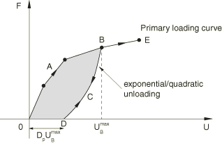
The model in Figure 31.2.10–7 illustrates an analytical unloading curve that is derived based on an energy dissipation factor, ![]() (fraction of energy that is dissipated at any displacement level) and a permanent deformation factor,
(fraction of energy that is dissipated at any displacement level) and a permanent deformation factor, ![]() . As the connector is loaded, the force follows the path given by the loading curve. If the connector is unloaded (for example, at point B), the force follows the unloading curve
. As the connector is loaded, the force follows the path given by the loading curve. If the connector is unloaded (for example, at point B), the force follows the unloading curve ![]() . The point D corresponds to the permanent deformation,
. The point D corresponds to the permanent deformation, ![]() . Reloading after unloading follows the unloading curve
. Reloading after unloading follows the unloading curve ![]() until the loading is such that the displacement becomes greater than
until the loading is such that the displacement becomes greater than ![]() , after which the loading path follows the loading curve. The arrows shown in Figure 31.2.10–7 illustrate the loading/unloading paths of this model.
, after which the loading path follows the loading curve. The arrows shown in Figure 31.2.10–7 illustrate the loading/unloading paths of this model.
The unloading response follows the loading curve when the calculated unloading curve lies above the loading curve to prevent energy generation and follows a zero force response when the unloading curve yields a negative response. In such cases the dissipated energy will be less than the value specified by the energy dissipation factor.
| Input File Usage: | Use the following option to define quadratic unloading behavior: |
*UNLOADING DATA, DEFINITION=QUADRATIC Use the following option to define exponential unloading behavior: *UNLOADING DATA, DEFINITION=EXPONENTIAL |
The model in Figure 31.2.10–8 illustrates an interpolated unloading response based on multiple unloading curves that intersect the primary loading curve at increasing values of forces/displacements. You can specify as many unloading curves as are necessary to define the unloading response. The first point of each unloading curve defines the permanent deformation if the connector is completely unloaded. The unloading curves are stored in normalized form so that they intersect the loading curve at a unit force for a unit displacement, and the interpolation occurs between these normalized curves. If unloading occurs from a maximum displacement for which an unloading curve is not specified, the unloading curve is interpolated from neighboring unloading curves. As the connector is loaded, the force follows the path given by the loading curve. If the connector is unloaded (for example, at point B), the force follows the unloading curve ![]() . Reloading after unloading follows the unloading path
. Reloading after unloading follows the unloading path ![]() until the loading is such that the displacement becomes greater than
until the loading is such that the displacement becomes greater than ![]() , after which the loading path follows the loading curve.
, after which the loading path follows the loading curve.
If the loading curve depends on the constitutive displacements/rotations in several component directions, the unloading curves also depends on the same component directions. The unloading curve also has the same temperature and field variable dependencies as the loading curve.
| Input File Usage: | *UNLOADING DATA, DEFINITION=INTERPOLATED CURVE |
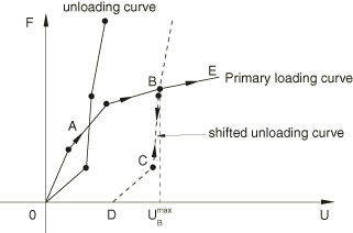
You can specify an unloading curve passing through the origin in addition to the loading curve. The actual unloading curve is obtained by horizontally shifting the user-specified unloading curve to pass through the point of unloading as shown in Figure 31.2.10–9. The permanent deformation upon complete unloading is the horizontal shift applied to the unloading curve.
If the loading curve depends on the constitutive displacements/rotations in several component directions, the unloading curve also depends on the same component directions. The unloading curve also has the same temperature and field variable dependencies as the loading curve.
| Input File Usage: | *UNLOADING DATA, DEFINITION=SHIFTED CURVE |
When appropriate, different uniaxial behavior models can be used in tension and compression. For example, a model with permanent deformation and exponential unloading in tension can be combined with a nonlinear elastic model in compression (see Figure 31.2.10–10).
The Abaqus output variables available for connectors are listed in “Abaqus/Standard output variable identifiers,” Section 4.2.1, and “Abaqus/Explicit output variable identifiers,” Section 4.2.2. The following output variables are of particular interest when defining uniaxial behavior in connectors:
CU | Connector relative displacements/rotations. |
CUF | Connector uniaxial forces/moments. |