Products: Abaqus/Standard Abaqus/Explicit Abaqus/CAE
The features described in this section allow the specification of generalized traction-separation behavior for surfaces. This behavior offers capabilities that are very similar to cohesive elements that are defined using a traction-separation law (see “Defining the constitutive response of cohesive elements using a traction-separation description,” Section 32.5.6). However, surface-based cohesive behavior is typically easier to define and allows simulation of a wider range of cohesive interactions, such as two “sticky” surfaces coming into contact during an analysis.
Surface-based cohesive behavior is primarily intended for situations in which the interface thickness is negligibly small. If the interface adhesive layer has a finite thickness and macroscopic properties (such as stiffness and strength) of the adhesive material are available, it may be more appropriate to model the response using conventional cohesive elements (see “Defining the constitutive response of cohesive elements using a continuum approach,” Section 32.5.5).
In Abaqus/Explicit the surface-based cohesive behavior framework can also be used to model crack propagation in initially partially bonded surfaces via linear elastic fracture mechanics principles (LEFM) as implemented using the Virtual Crack Closure Technique (VCCT).
Surface-based cohesive behavior:
is defined as a surface interaction property;
can be used to model the delamination at interfaces directly in terms of traction versus separation;
can be used to model “sticky” contact (i.e., surfaces or parts of surfaces that are not initially in contact may bond on coming into contact; subsequently the bond may damage and fail);
can be restricted to surface regions that are initially in contact and, in Abaqus/Standard, to portions of surface regions that are initially in contact;
allows specification of cohesive data such as the fracture energy as a function of the ratio of normal to shear displacements (mode mix) at the interface;
assumes a linear elastic traction-separation law prior to damage;
assumes that failure of the cohesive bond is characterized by progressive degradation of the cohesive stiffness, which is driven by a damage process (in Abaqus/Explicit brittle fracture can also be modeled using a VCCT fracture crierion);
allows specification of post-failure cohesive behavior if failed nodes re-enter contact;
is implemented within the general contact algorithmic framework in Abaqus/Explicit and within the contact pair framework in Abaqus/Standard;
can be used to enforce “rough friction” surface interactions, the “no separation” contact relationship, or a combined “no separation and rough friction” behavior within the general contact framework in Abaqus/Explicit;
is enforced only for node-to-face contact interactions in Abaqus/Explicit and is not available for edge-to-edge and node-to-analytical rigid surface contact interactions;
cannot be used in a coupled Eulerian-Lagrangian analysis in Abaqus/Explicit; and
can be used for all Abaqus/Standard contact formulations except the finite sliding, surface-to-surface formulation.
Cohesive behavior in Abaqus/Explicit is defined as part of the surface interaction properties that are assigned to the applicable surfaces. General contact must be defined for the model.
| Input File Usage: | Use the following options to define cohesive behavior between two surfaces in a general contact definition: |
*SURFACE INTERACTION, NAME=name *COHESIVE BEHAVIOR *CONTACT *CONTACT PROPERTY ASSIGNMENT surface1, surface2, name |
| Abaqus/CAE Usage: | Use the following option to define cohesive behavior between two surfaces: |
Interaction module: contact property editor: Mechanical Use the following option to define contact between two surfaces: Interaction module: interaction editor: General contact (Explicit): specify Contact interaction property |
In Abaqus/Explicit overconstraints can arise in certain situations if the balanced master-slave formulation is enforced in addition to the cohesive constraint. To prevent this from occurring, a pure master-slave formulation is enforced for surfaces with cohesive behavior in Abaqus/Explicit. If cohesive behavior is defined between two surfaces, the first surface defined in the contact property assignment is treated as a slave surface and the second surface as its corresponding master surface. For contact interactions between the cohesive surfaces and other parts of the general contact domain, the default contact formulation (balanced master-slave) is applicable, unless a nondefault general contact formulation has been defined (see “Contact formulation for general contact in Abaqus/Explicit,” Section 37.2.1). The surface-based cohesive behavior is available only for node-to-face contact interactions; it is not available for edge-to-edge interactions. Hence, it is not possible to define surface-based cohesion between edges of beam and truss elements. In addition, contact definitions related to thermal interactions are ignored when surface-based cohesive behavior is defined.
Care should be exercised when cohesive behavior is used in conjunction with stacked conventional shell elements. Depending on the load case, the specialized contact formulation may lead to approximate normal contact forces, which in turn may induce approximate transverse shear behavior in the stacked shells that affect the bending behavior of the stack. Continuum shells should be used instead of conventional shells in such modeling scenarios.
In many debonding applications using cohesive surfaces, it may be desirable to begin the analysis with the surfaces just touching each other. This requires the resolution of initial overclosures and gaps between the surfaces at the start of the analysis to ensure that the slave nodes are precisely in contact with the master surface. In Abaqus/Explicit small initial overclosures are set to zero by default. To resolve large initial overclosures or to close initial gaps between the surfaces, an appropriate contact clearance specification may be defined, as explained in “Controlling initial contact status for general contact in Abaqus/Explicit,” Section 35.4.4. Since a pure-master slave formulation is enforced for cohesive surfaces, only nodes of the slave surface will undergo strain-free corrections to resolve any initial overclosures or gaps with their master facets; the nodes of the master facets will not be moved.
Cohesive behavior in Abaqus/Standard is defined as part of the surface interaction properties that are assigned to a contact pair. Cohesive behavior cannot be assigned to contact pairs using the finite sliding, surface-to-surface formulation (see “Contact formulations in Abaqus/Standard,” Section 37.1.1).
| Input File Usage: | Use the following options to define cohesive behavior between the surfaces in a contact pair: |
*SURFACE INTERACTION, NAME=name *COHESIVE BEHAVIOR *CONTACT PAIR, INTERACTION=name surface1, surface2 |
| Abaqus/CAE Usage: | Use the following option to define cohesive behavior between two surfaces: |
Interaction module: contact property editor: Mechanical Use the following option to define surface-to-surface contact between two surfaces: Interaction module: interaction editor: Surface-to-surface contact (Standard): Bonding tabbed page: specify Contact interaction property |
As discussed above, it is often desirable in debonding applications for the cohesive surfaces to begin the analysis just touching each other. Abaqus/Standard offers some tools for adjusting slave nodes in a contact pair so that they precisely contact the master surface, thereby eliminating initial overclosures and gaps. If nodes are not adjusted, even an extremely small initial gap will cause the contact constraints to be initialized to inactive and, thus, not cohered. These tools are described in “Adjusting initial surface positions and specifying initial clearances in Abaqus/Standard contact pairs,” Section 35.3.5.
By default, cohesive constraint forces can potentially act on all nodes of the surfaces for which cohesive behavior is defined. Slave nodes that are initially contacting the master surface can experience cohesive forces at the start of the analysis, and slave nodes that are not initially contacting the master surface can experience cohesive forces if they contact the master surface during the analysis. There may, however, be situations where it is desirable to enforce cohesive behavior only for portions of surfaces that are contacting at the start of the analysis.
As part of the cohesive behavior definition, you can indicate that only those nodes that are in contact with the master surface at the start of the step should experience cohesive forces. Any new contacts that occur during the step will not experience cohesive constraint forces; they will be modeled only as compressive contact.
| Input File Usage: | *COHESIVE BEHAVIOR, ELIGIBILITY=ORIGINAL CONTACTS |
| Abaqus/CAE Usage: | Interaction module: contact property editor: Mechanical |
In Abaqus/Standard you can specify a subset of initially slave nodes that should experience cohesive forces. Strain-free adjustments will be made for those nodes initially not in contact but specified in the node set. All slave nodes outside of this set (including those that are initially contacting the master surface) will experience only compressive contact forces over the course of the analysis. This method is particularly useful for modeling crack propagation along an existing fault line.
| Input File Usage: | Use both of the following options: |
*INITIAL CONDITIONS, TYPE=CONTACT *COHESIVE BEHAVIOR, ELIGIBILITY=SPECIFIED CONTACTS |
| Abaqus/CAE Usage: | Interaction module: contact property editor: Mechanical |
Interaction module: interaction editor: Bonding tabbed page: Limit bonding to slave nodes in sub-set |
In the contact normal direction, the pressure overclosure relationship governing the compressive behavior between the surfaces does not interact with the cohesive behavior, since they each describe the interaction between the surfaces in a different contact regime. The pressure overclosure relationship governs the behavior only when a slave node is “closed” (i.e., it is in contact with the master surface); the cohesive behavior contributes to the contact normal stress only when a slave node is “open” (i.e., not in contact). In the case of “sticky” cohesive behavior—where the two surfaces are not initially in contact—cohesive effects are activated in the increment after the slave node status changes from open to closed.
In the shear direction, if the cohesive stiffness is undamaged, it is assumed that the cohesive model is active and the friction model is dormant. Any tangential slip is assumed to be purely elastic in nature and is resisted by the cohesive strength of the bond, resulting in shear forces. If damage has been defined, the cohesive contribution to the shear stresses starts degrading with damage evolution. Once the cohesive stiffness starts degrading, the friction model activates and begins contributing to the shear stresses. The elastic stick stiffness of the friction model is ramped up in proportion to the degradation of the elastic cohesive stiffness. Prior to the ultimate failure of the cohesive bond, and following the initiation of the degradation of the cohesive bond, the shear stress is a combination of the cohesive contribution and the contribution from the friction model. Once maximum degradation has been reached, the cohesive contribution to the shear stresses is zero, and the only contribution to the shear stresses is from the friction model.
The formulae and laws that govern cohesive surface behavior are very similar to those used for cohesive elements with traction-separation constitutive behavior (“Defining the constitutive response of cohesive elements using a traction-separation description,” Section 32.5.6). The similarities extend to the linear elastic traction-separation model, damage initiation criteria, and damage evolution laws.
However, it is important to recognize that damage in surface-based cohesive behavior is an interaction property, not a material property. Concepts of strain and displacement (used in behavior model formulae for cohesive elements) are reinterpreted as contact separations; contact separations are the relative displacements between the nodes on the slave surface and their corresponding projection points on the master surface along the contact normal and shear directions. Stresses are defined for surface-based cohesive behavior as the cohesive forces acting along the contact normal and shear directions divided by the current area at each contact point.
The specifics of the surface-based cohesive behavior model are discussed in the sections that follow.
The available traction-separation model in Abaqus assumes initially linear elastic behavior (see “Defining elasticity in terms of tractions and separations for cohesive elements” in “Linear elastic behavior,” Section 22.2.1) followed by the initiation and evolution of damage. The elastic behavior is written in terms of an elastic constitutive matrix that relates the normal and shear stresses to the normal and shear separations across the interface.
The nominal traction stress vector, ![]() , consists of three components (two components in two-dimensional problems):
, consists of three components (two components in two-dimensional problems): ![]() ,
, ![]() , and (in three-dimensional problems)
, and (in three-dimensional problems) ![]() , which represent the normal (along the local 3-direction in three dimensions and along the local 2-direction in two dimensions) and the two shear tractions (along the local 1- and 2-directions in three dimensions and along the local 1-direction in two dimensions), respectively. The corresponding separations are denoted by
, which represent the normal (along the local 3-direction in three dimensions and along the local 2-direction in two dimensions) and the two shear tractions (along the local 1- and 2-directions in three dimensions and along the local 1-direction in two dimensions), respectively. The corresponding separations are denoted by ![]() ,
, ![]() , and
, and ![]() . The elastic behavior can then be written as
. The elastic behavior can then be written as
The simplest specification of cohesive behavior generates contact penalties that enforce the cohesive constraint in both normal and tangential directions. By default, the normal and tangential stiffness components will not be coupled: pure normal separation by itself does not give rise to cohesive forces in the shear directions, and pure shear slip with zero normal separation does not give rise to any cohesive forces in the normal direction.
For uncoupled traction-separation behavior, the terms ![]() ,
, ![]() , and
, and ![]() must be defined, as well as any dependencies on temperature or field variables. If these terms are not defined, Abaqus uses default contact penalties to model the traction-separation behavior.
must be defined, as well as any dependencies on temperature or field variables. If these terms are not defined, Abaqus uses default contact penalties to model the traction-separation behavior.
| Input File Usage: | *COHESIVE BEHAVIOR, TYPE=UNCOUPLED (default) |
| Abaqus/CAE Usage: | Interaction module: contact property editor: Mechanical |
In its full generality, the elasticity matrix provides fully coupled behavior between all components of the traction vector and separation vector and can depend on temperature and/or field variables. All terms in the matrix must be defined for coupled traction-separation behavior.
| Input File Usage: | *COHESIVE BEHAVIOR, TYPE=COUPLED |
| Abaqus/CAE Usage: | Interaction module: contact property editor: Mechanical |
To restrict the cohesive constraint to act along the contact normal direction only, define uncoupled cohesive behavior and specify zero values for the shear stiffness components, ![]() and
and ![]() . Alternatively, if only tangential cohesive constraints are to be enforced, the normal stiffness term,
. Alternatively, if only tangential cohesive constraints are to be enforced, the normal stiffness term, ![]() , can be set to zero, in which case the normal “separations” will not be constrained. Normal compressive forces are resisted as per the usual contact behavior.
, can be set to zero, in which case the normal “separations” will not be constrained. Normal compressive forces are resisted as per the usual contact behavior.
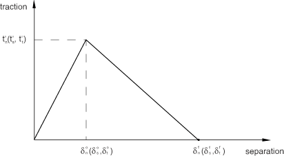
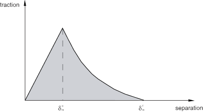
Damage modeling allows you to simulate the degradation and eventual failure of the bond between two cohesive surfaces. The failure mechanism consists of two ingredients: a damage initiation criterion and a damage evolution law. The initial response is assumed to be linear as discussed above. However, once a damage initiation criterion is met, damage can occur according to a user-defined damage evolution law. Figure 36.1.10–1 shows a typical traction-separation response with a failure mechanism. If the damage initiation criterion is specified without a corresponding damage evolution model, Abaqus evaluates the damage initiation criterion for output purposes only; there is no effect on the response of the cohesive surfaces (i.e., no damage will occur). Cohesive surfaces do not undergo damage under pure compression.
Damage of the traction-separation response for cohesive surfaces is defined within the same general framework used for conventional materials (see “Progressive damage and failure,” Section 24.1.1), except the damage behavior is specified as part of the interaction properties for the surfaces. Multiple damage response mechanisms are not available for cohesive surfaces: cohesive surfaces can have only one damage initiation criterion and only one damage evolution law.
| Input File Usage: | Use the following options to define damage initiation and damage evolution for cohesive surfaces: |
*SURFACE INTERACTION, NAME=name *COHESIVE BEHAVIOR *DAMAGE INITIATION *DAMAGE EVOLUTION |
| Abaqus/CAE Usage: | Interaction module: contact property editor: Mechanical |
Damage initiation refers to the beginning of degradation of the cohesive response at a contact point. The process of degradation begins when the contact stresses and/or contact separations satisfy certain damage initiation criteria that you specify. Several damage initiation criteria are available and are discussed below.
Each damage initiation criterion also has an output variable associated with it to indicate whether the criterion is met. A value of 1 or higher indicates that the initiation criterion has been met. Damage initiation criteria that do not have an associated evolution law affect only output. Thus, you can use these criteria to evaluate the propensity of the material to undergo damage without actually modeling the damage process (i.e., without actually specifying damage evolution).
In the discussion below, ![]() ,
, ![]() , and
, and ![]() represent the peak values of the contact stress when the separation is either purely normal to the interface or purely in the first or the second shear direction, respectively. Likewise,
represent the peak values of the contact stress when the separation is either purely normal to the interface or purely in the first or the second shear direction, respectively. Likewise, ![]() ,
, ![]() , and
, and ![]() represent the peak values of the contact separation, when the separation is either purely along the contact normal or purely in the first or the second shear direction, respectively. The symbol
represent the peak values of the contact separation, when the separation is either purely along the contact normal or purely in the first or the second shear direction, respectively. The symbol ![]() used in the discussion below represents the Macaulay bracket with the usual interpretation. The Macaulay brackets are used to signify that a purely compressive displacement (i.e., a contact penetration) or a purely compressive stress state does not initiate damage.
used in the discussion below represents the Macaulay bracket with the usual interpretation. The Macaulay brackets are used to signify that a purely compressive displacement (i.e., a contact penetration) or a purely compressive stress state does not initiate damage.
Damage is assumed to initiate when the maximum contact stress ratio (as defined in the expression below) reaches a value of one. This criterion can be represented as
![]()
| Input File Usage: | *DAMAGE INITIATION, CRITERION=MAXS |
| Abaqus/CAE Usage: | Interaction module: contact property editor: Mechanical |
Damage is assumed to initiate when the maximum separation ratio (as defined in the expression below) reaches a value of one. This criterion can be represented as
![]()
| Input File Usage: | *DAMAGE INITIATION, CRITERION=MAXU |
| Abaqus/CAE Usage: | Interaction module: contact property editor: Mechanical |
Damage is assumed to initiate when a quadratic interaction function involving the contact stress ratios (as defined in the expression below) reaches a value of one. This criterion can be represented as
![]()
| Input File Usage: | *DAMAGE INITIATION, CRITERION=QUADS |
| Abaqus/CAE Usage: | Interaction module: contact property editor: Mechanical |
Damage is assumed to initiate when a quadratic interaction function involving the separation ratios (as defined in the expression below) reaches a value of one. This criterion can be represented as
![]()
| Input File Usage: | *DAMAGE INITIATION, CRITERION=QUADU |
| Abaqus/CAE Usage: | Interaction module: contact property editor: Mechanical |
The damage evolution law describes the rate at which the cohesive stiffness is degraded once the corresponding initiation criterion is reached. The general framework for describing the evolution of damage in bulk materials (as opposed to interfaces modeled using cohesive surfaces) is described in “Damage evolution and element removal for ductile metals,” Section 24.2.3. Conceptually, similar ideas apply for describing damage evolution in cohesive surfaces.
A scalar damage variable, D, represents the overall damage at the contact point. It initially has a value of 0. If damage evolution is modeled, D monotonically evolves from 0 to 1 upon further loading after the initiation of damage. The contact stress components are affected by the damage according to
![]()
![]()
![]()
To describe the evolution of damage under a combination of normal and shear separations across the interface, it is useful to introduce an effective separation (Camanho and Davila, 2002) defined as
![]()
The relative proportions of normal and shear separations at a contact point define the mode mix at the point. Abaqus uses two measures of mode mix, one based on energies and the other based on tractions. You can choose one of these measures when you specify the mode dependence of the damage evolution process. Denoting by ![]() ,
, ![]() , and
, and ![]() the work done by the tractions and their conjugate separations in the normal, first, and second shear directions, respectively, and defining
the work done by the tractions and their conjugate separations in the normal, first, and second shear directions, respectively, and defining ![]() , the mode-mix definitions based on energies are as follows:
, the mode-mix definitions based on energies are as follows:
![]()
![]()
![]()
The corresponding definitions of the mode mix based on traction components are given by
![]()
![]()
The mode-mix ratios defined in terms of energies and tractions can be quite different in general. The following example illustrates this point. In terms of energies a separation in the purely normal direction is one for which ![]() and
and ![]() , irrespective of the values of the normal and the shear tractions. In particular, for coupled traction-separation behavior both the normal and shear tractions may be nonzero for a purely normal separation. For this case the definition of mode mix based on energies would indicate a purely normal separation, while the definition based on tractions would suggest a mix of both normal and shear separation.
, irrespective of the values of the normal and the shear tractions. In particular, for coupled traction-separation behavior both the normal and shear tractions may be nonzero for a purely normal separation. For this case the definition of mode mix based on energies would indicate a purely normal separation, while the definition based on tractions would suggest a mix of both normal and shear separation.
There are two components to the definition of damage evolution. The first component involves specifying either the effective separation at complete failure, ![]() , relative to the effective separation at the initiation of damage,
, relative to the effective separation at the initiation of damage, ![]() ; or the energy dissipated due to failure,
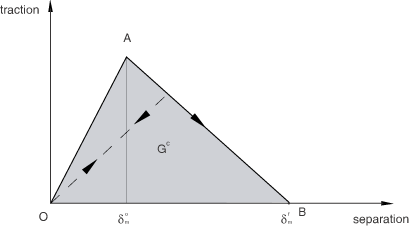
; or the energy dissipated due to failure, ![]() (see Figure 36.1.10–3). The second component to the definition of damage evolution is the specification of the nature of the evolution of the damage variable, D, between initiation of damage and final failure. This can be done by either defining linear or exponential softening laws or specifying D directly as a tabular function of the effective separation relative to the effective separation at damage initiation. The data described above will in general be functions of the mode mix, temperature, and/or field variables.
(see Figure 36.1.10–3). The second component to the definition of damage evolution is the specification of the nature of the evolution of the damage variable, D, between initiation of damage and final failure. This can be done by either defining linear or exponential softening laws or specifying D directly as a tabular function of the effective separation relative to the effective separation at damage initiation. The data described above will in general be functions of the mode mix, temperature, and/or field variables.
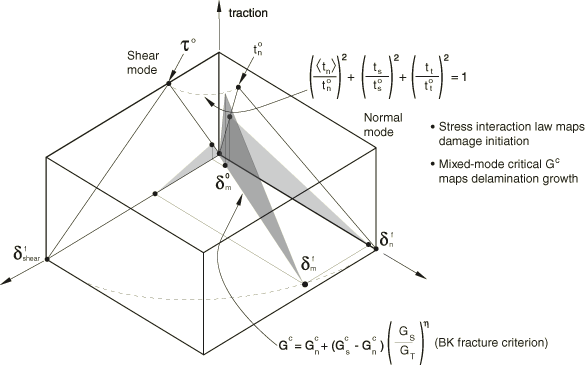
Figure 36.1.10–4 is a schematic representation of the dependence of damage initiation and evolution on the mode mix for a traction-separation response with isotropic shear behavior. The figure shows the traction on the vertical axis and the magnitudes of the normal and the shear separations along the two horizontal axes. The unshaded triangles in the two vertical coordinate planes represent the response under pure normal and pure shear separation, respectively. All intermediate vertical planes (that contain the vertical axis) represent the damage response under mixed-mode conditions with different mode mixes. The dependence of the damage evolution data on the mode mix can be defined either in tabular form or, in the case of an energy-based definition, analytically. The manner in which the damage evolution data are specified as a function of the mode mix is discussed later in this section.
Unloading subsequent to damage initiation is always assumed to occur linearly toward the origin of the traction-separation plane, as shown in Figure 36.1.10–3. Reloading subsequent to unloading also occurs along the same linear path until the softening envelope (line AB) is reached. Once the softening envelope is reached, further reloading follows this envelope as indicated by the arrow in Figure 36.1.10–3.
| Input File Usage: | Use the following option to use the mode-mix definition based on energies: |
*DAMAGE EVOLUTION, MODE MIX RATIO=ENERGY Use the following option to use the mode-mix definition based on tractions: *DAMAGE EVOLUTION, MODE MIX RATIO=TRACTION |
| Abaqus/CAE Usage: | Interaction module: contact property editor: Mechanical |
You specify the quantity ![]() (i.e., the effective separation at complete failure,
(i.e., the effective separation at complete failure, ![]() , relative to the effective separation at damage initiation,
, relative to the effective separation at damage initiation, ![]() , as shown in Figure 36.1.10–3) as a tabular function of the mode mix, temperature, and/or field variables. In addition, you also choose either a linear or an exponential softening law that defines the detailed evolution (between initiation and complete failure) of the damage variable, D, as a function of the effective separation beyond damage initiation. Alternatively, instead of using linear or exponential softening, you can specify the damage variable, D, directly as a tabular function of the effective separation after the initiation of damage,
, as shown in Figure 36.1.10–3) as a tabular function of the mode mix, temperature, and/or field variables. In addition, you also choose either a linear or an exponential softening law that defines the detailed evolution (between initiation and complete failure) of the damage variable, D, as a function of the effective separation beyond damage initiation. Alternatively, instead of using linear or exponential softening, you can specify the damage variable, D, directly as a tabular function of the effective separation after the initiation of damage, ![]() ; mode mix; temperature; and/or field variables.
; mode mix; temperature; and/or field variables.
For linear softening (see Figure 36.1.10–3) Abaqus uses an evolution of the damage variable, D, that reduces (in the case of damage evolution under a constant mode mix, temperature, and field variables) to the following expression:
![]()
| Input File Usage: | Use the following option to specify linear damage evolution: |
*DAMAGE EVOLUTION, TYPE=DISPLACEMENT, SOFTENING=LINEAR |
| Abaqus/CAE Usage: | Interaction module: contact property editor: Mechanical |
For exponential softening (see Figure 36.1.10–5) Abaqus uses an evolution of the damage variable, D, that reduces (in the case of damage evolution under a constant mode mix, temperature, and field variables) to
| Input File Usage: | Use the following option to specify exponential softening: |
*DAMAGE EVOLUTION, TYPE=DISPLACEMENT, SOFTENING=EXPONENTIAL |
| Abaqus/CAE Usage: | Interaction module: contact property editor: Mechanical |
For tabular softening you define the evolution of D directly in tabular form. D must be specified as a function of the effective separation relative to the effective separation at initiation, mode mix, temperature, and/or field variables.
| Input File Usage: | Use the following option to define the damage variable directly in tabular form: |
*DAMAGE EVOLUTION, TYPE=DISPLACEMENT, SOFTENING=TABULAR |
| Abaqus/CAE Usage: | Interaction module: contact property editor: Mechanical |
Damage evolution can be defined based on the energy that is dissipated as a result of the damage process, also called the fracture energy. The fracture energy is equal to the area under the traction-separation curve (see Figure 36.1.10–3). You specify the fracture energy as a property of the cohesive interaction and choose either a linear or an exponential softening behavior. Abaqus ensures that the area under the linear or the exponential damaged response is equal to the fracture energy.
The dependence of the fracture energy on the mode mix can be specified either directly in tabular form or by using analytical forms as described below. When the analytical forms are used, the mode-mix ratio is assumed to be defined in terms of energies.
The simplest way to define the dependence of the fracture energy is to specify it directly as a function of the mode mix in tabular form.
| Input File Usage: | Use the following option to specify fracture energy as a function of the mode mix in tabular form: |
*DAMAGE EVOLUTION, TYPE=ENERGY, MIXED MODE BEHAVIOR=TABULAR |
| Abaqus/CAE Usage: | Interaction module: contact property editor: Contact: Mechanical |
The dependence of the fracture energy on the mode mix can be defined based on a power law fracture criterion. The power law criterion states that failure under mixed-mode conditions is governed by a power law interaction of the energies required to cause failure in the individual (normal and two shear) modes. It is given by
![]()
![]()
| Input File Usage: | Use the following option to define the fracture energy as a function of the mode mix using the analytical power law fracture criterion: |
*DAMAGE EVOLUTION, TYPE=ENERGY, MIXED MODE BEHAVIOR=POWER LAW, POWER= |
| Abaqus/CAE Usage: | Interaction module: contact property editor: Mechanical |
The Benzeggagh-Kenane fracture criterion (Benzeggagh and Kenane, 1996) is particularly useful when the critical fracture energies during separation purely along the first and the second shear directions are the same; i.e., ![]() . It is given by
. It is given by
![]()
| Input File Usage: | Use the following option to define the fracture energy as a function of the mode mix using the analytical BK fracture criterion: |
*DAMAGE EVOLUTION, TYPE=ENERGY, MIXED MODE BEHAVIOR=BK, POWER= |
| Abaqus/CAE Usage: | Interaction module: contact property editor: Mechanical |
For linear softening (see Figure 36.1.10–3) Abaqus uses an evolution of the damage variable, D, that reduces to
![]()
| Input File Usage: | Use the following option to specify linear damage evolution: |
*DAMAGE EVOLUTION, TYPE=ENERGY, SOFTENING=LINEAR |
| Abaqus/CAE Usage: | Interaction module: contact property editor: Mechanical |
For exponential softening Abaqus uses an evolution of the damage variable, D, that reduces to
![]()
| Input File Usage: | Use the following option to specify exponential softening: |
*DAMAGE EVOLUTION, TYPE=ENERGY, SOFTENING=EXPONENTIAL |
| Abaqus/CAE Usage: | Interaction module: contact property editor: Mechanical |
As discussed earlier, the data defining the evolution of damage at the cohesive interface can be tabular functions of the mode mix. The manner in which this dependence must be defined in Abaqus is outlined below for mode-mix definitions based on energy and traction, respectively. In the following discussion it is assumed that the evolution is defined in terms of energy. Similar observations can also be made for evolution definitions based on effective separation.
For an energy-based definition of mode mix, in the most general case of a three-dimensional state of separation with anisotropic shear behavior the fracture energy, ![]() , must be defined as a function of
, must be defined as a function of ![]() and
and ![]() . The quantity
. The quantity ![]() is a measure of the fraction of the total separation that is shear, while
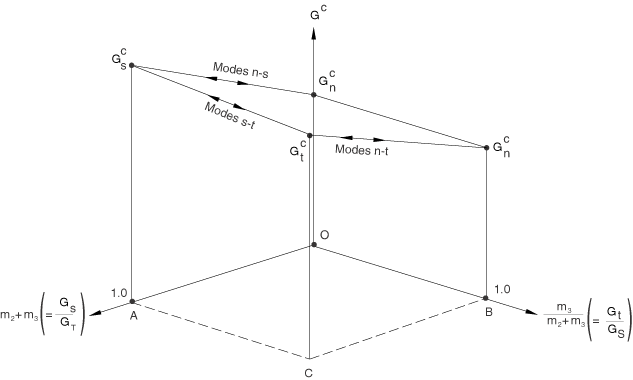
is a measure of the fraction of the total separation that is shear, while ![]() is a measure of the fraction of the total shear separation that is in the second shear direction. Figure 36.1.10–6 shows a schematic of the fracture energy versus mode-mix behavior.
is a measure of the fraction of the total shear separation that is in the second shear direction. Figure 36.1.10–6 shows a schematic of the fracture energy versus mode-mix behavior.
For a two-dimensional problem ![]() needs to be defined as a function of
needs to be defined as a function of ![]() (
(![]() in this case) only. The data column corresponding to
in this case) only. The data column corresponding to ![]() must be left blank. Hence, essentially only one “data block” is needed.
must be left blank. Hence, essentially only one “data block” is needed.
For a three-dimensional problem with isotropic shear response, the shear behavior is defined by the sum ![]() and not by the individual values of
and not by the individual values of ![]() and
and ![]() . Therefore, in this case a single “data block” (the “data block” for
. Therefore, in this case a single “data block” (the “data block” for ![]() ) also suffices to define the fracture energy as a function of the mode mix.
) also suffices to define the fracture energy as a function of the mode mix.
In the most general case of three-dimensional problems with anisotropic shear behavior, several “data blocks” would be needed. As discussed earlier, each “data block” would contain ![]() versus
versus ![]() at a fixed value of
at a fixed value of ![]() . In each “data block”
. In each “data block” ![]() can vary between 0 and 1.0. The case
can vary between 0 and 1.0. The case ![]() (the first data point in any “data block”), which corresponds to a purely normal mode, can never be achieved when
(the first data point in any “data block”), which corresponds to a purely normal mode, can never be achieved when ![]() (i.e., the only valid point on line OB in Figure 36.1.10–6 is the point O, which corresponds to a purely normal separation). However, in the tabular definition of the fracture energy as a function of mode mix, this point simply serves to set a limit that ensures a continuous change in fracture energy as a purely normal state is approached from various combinations of normal and shear separations. Hence, the fracture energy of the first data point in each “data block” must always be set equal to the fracture energy in a purely normal separation (
(i.e., the only valid point on line OB in Figure 36.1.10–6 is the point O, which corresponds to a purely normal separation). However, in the tabular definition of the fracture energy as a function of mode mix, this point simply serves to set a limit that ensures a continuous change in fracture energy as a purely normal state is approached from various combinations of normal and shear separations. Hence, the fracture energy of the first data point in each “data block” must always be set equal to the fracture energy in a purely normal separation (![]() ).
).
As an example of the anisotropic shear case, consider that you want to input three “data blocks” corresponding to fixed values of ![]() 0., 0.2, and 1.0, respectively. For each of the three “data blocks,” the first data point must be
0., 0.2, and 1.0, respectively. For each of the three “data blocks,” the first data point must be ![]() for the reasons discussed above. The rest of the data points in each “data block” define the variation of the fracture energy with increasing proportions of shear separation.
for the reasons discussed above. The rest of the data points in each “data block” define the variation of the fracture energy with increasing proportions of shear separation.
The fracture energy needs to be specified in tabular form of ![]() versus
versus ![]() and
and ![]() . Thus,
. Thus, ![]() needs to be specified as a function of
needs to be specified as a function of ![]() at various fixed values of
at various fixed values of ![]() . A “data block” in this case corresponds to a set of data for
. A “data block” in this case corresponds to a set of data for ![]() versus
versus ![]() , at a fixed value of
, at a fixed value of ![]() . In each “data block”
. In each “data block” ![]() may vary from 0 (purely normal separation) to 1 (purely shear separation). An important restriction is that each data block must specify the same value of the fracture energy for
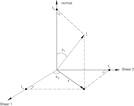
may vary from 0 (purely normal separation) to 1 (purely shear separation). An important restriction is that each data block must specify the same value of the fracture energy for ![]() . This restriction ensures that the energy required for fracture as the traction vector approaches the normal direction does not depend on the orientation of the projection of the traction vector on the shear plane (see Figure 36.1.10–2).
. This restriction ensures that the energy required for fracture as the traction vector approaches the normal direction does not depend on the orientation of the projection of the traction vector on the shear plane (see Figure 36.1.10–2).
Models exhibiting various forms of softening behavior and stiffness degradation often lead to severe convergence difficulties in Abaqus/Standard. Viscous regularization of the constitutive equations defining surface-based cohesive behavior can be used to overcome some of these convergence difficulties. This technique is also applicable to cohesive elements, fastener damage, and the concrete material model in Abaqus/Standard. Viscous regularization damping causes the tangent stiffness matrix that defines the contact stresses to be positive for sufficiently small time increments.
The approximate amount of energy associated with viscous regularization over the whole model is available using output variable ALLVD.
| Input File Usage: | *DAMAGE STABILIZATION |
| Abaqus/CAE Usage: | Interaction module: contact property editor: Mechanical |
Two types of post-failure behavior can be specified to define the cohesive behavior at a node on the slave surface after the maximum degradation value, ![]() , has been reached at the node.
, has been reached at the node.
By default, once fully degraded, normal contact behavior is enforced at the node and no further cohesive constraints are enforced. If the slave node re-enters contact, penetrations will give rise to compressive contact stresses, and frictional stresses will be applied in the shear directions according to the prescribed friction model, if any. Separations can occur without giving rise to any cohesive stresses.
In some situations it may be desirable to enforce cohesive behavior again if a slave node re-enters contact, even after maximum degradation has been reached. For cohesive behavior allowing repeated contacts, the overall damage variable will be re-initialized to zero when a failed slave node re-enters contact. Subsequently, normal separations may give rise to tensile cohesive stresses, and shear separations may give rise to tangential cohesive stresses in accordance with the type of cohesive behavior defined. Further loading can again cause the cohesive stresses to undergo progressive damage, degrade, and fail.
| Input File Usage: | Use the following option to enforce cohesive behavior subsequent to maximum degradation: |
*COHESIVE BEHAVIOR, REPEATED CONTACTS |
| Abaqus/CAE Usage: | Interaction module: contact property editor: Mechanical |
In Abaqus/Explicit, the surface-based cohesive behavior framework can be used to model brittle crack propagation problems based on linear elastic fracture mechanics principles. The Virtual Crack Closure Technique (VCCT) fracture criterion can be used to model crack propagation in initially partially bonded surfaces. A detailed discussion of this topic can be found in “Crack propagation analysis,” Section 11.4.3.
The VCCT fracture criterion cannot be combined with a damage-based surface behavior of the traction-separation response. However, you can use a surface-based VCCT fracture criterion in conjunction with cohesive elements. VCCT could model brittle failure/crack propagation while the cohesive elements could model other aspects of the bonded interface such as stitches.
| Input File Usage: | Use the following options to enforce cohesive behavior subsequent to maximum degradation: |
*COHESIVE BEHAVIOR *FRACTURE CRITERION, TYPE= VCCT |
As described above, the formulation used for surface-based cohesive behavior is very similar to that for cohesive elements with traction-separation response. However, certain differences exist.
Interface thickness effects are never considered for cohesive surfaces; in cohesive elements with traction-separation response, thickness effects can be incorporated by either specifying a nonzero thickness for the interface or by requiring the initial constitutive thickness to be determined from the nodal coordinates of the cohesive elements. Since thickness effects are not considered for cohesive surfaces, material properties used to describe the constitutive response for traction-separation cohesive elements with thickness effects may not be directly reusable for cohesive surfaces.
For cohesive surfaces the cohesive constraint is enforced at each slave node; in cohesive elements the cohesive constraints are calculated at the material points (for the locations of material points in cohesive elements, see “Two-dimensional cohesive element library,” Section 32.5.8, and “Three-dimensional cohesive element library,” Section 32.5.9). Hence for cohesive surfaces, refining the slave surface as compared to the master surface will likely lead to improved constraint satisfaction and more accurate results.
In addition to the standard output identifiers available in Abaqus (“Abaqus/Standard output variable identifiers,” Section 4.2.1, and “Abaqus/Explicit output variable identifiers,” Section 4.2.2), the following variables have special meaning for cohesive surfaces with traction-separation behavior:
CSDMG | Overall value of the scalar damage variable, D. |
CSMAXSCRT | This variable indicates whether the maximum contact stress damage initiation criterion has been satisfied at a contact point. It is evaluated as |
CSMAXUCRT | This variable indicates whether the maximum separation damage initiation criterion has been satisfied at a contact point. It is evaluated as |
CSQUADSCRT | This variable indicates whether the quadratic contact stress damage initiation criterion has been satisfied at a contact point. It is evaluated as |
CSQUADUCRT | This variable indicates whether the quadratic separation damage initiation criterion has been satisfied at a contact point. It is evaluated as |
For the variables above that indicate whether a certain damage initiation criterion has been satisfied or not, a value that is less than 1.0 indicates that the criterion has not been satisfied, while a value of 1.0 indicates that the criterion has been satisfied. If damage evolution is specified for this criterion, the maximum value of this variable does not exceed 1.0.
Benzeggagh, M. L., and M. Kenane, “Measurement of Mixed-Mode Delamination Fracture Toughness of Unidirectional Glass/Epoxy Composites with Mixed-Mode Bending Apparatus,” Composites Science and Technology, vol. 56, pp. 439–449, 1996.
Camanho, P. P., and C. G. Davila, “Mixed-Mode Decohesion Finite Elements for the Simulation of Delamination in Composite Materials,” NASA/TM-2002–211737, pp. 1–37, 2002.