Products: Abaqus/Standard Abaqus/CAE
“Defining general contact interactions in Abaqus/Standard,” Section 35.2.1
“Defining general contact,” Section 15.13.1 of the Abaqus/CAE User's Manual
“Defining surface-to-surface contact,” Section 15.13.7 of the Abaqus/CAE User's Manual
“Using contact and constraint detection,” Section 15.16 of the Abaqus/CAE User's Manual
This section highlights the difficulties that are most commonly encountered when modeling contact interactions with Abaqus/Standard. Recommendations on how to circumvent these problems are presented.
It is important to understand how Abaqus/Standard interprets and resolves contact conditions at the start of a step or analysis. If necessary, you can check initial contact conditions in the message file (see “The Abaqus/Standard message file” in “Output,” Section 4.1.1). Unintentional contact openings or overclosures can lead to poor interpretations of surface geometry, unintentional motion in a model, and failure of an analysis to converge.
When modeling the contact between two faceted surfaces, it is often possible for small gaps or penetrations to occur at individual nodes. This problem is particularly common when the two surfaces have dissimilar meshes. Abaqus/Standard uses two default methods for dealing with initial penetrations:
In general contact small initial overclosures are automatically adjusted to remove the penetrations.
In contact pairs initial overclosures are interpreted as interference fits and resolved accordingly (see “Resolving large interference fits” below).
The small-sliding contact tracking approach is more sensitive than the finite-sliding tracking approach to initial local gaps at the contact interface. In small-sliding contact each slave node interacts with a contact plane defined from the finite element approximation of the master surface, as discussed in “Contact formulations in Abaqus/Standard,” Section 37.1.1. Abaqus/Standard can define these planes only when each slave node can be projected onto the master surface. Having these slave nodes start the simulation contacting the master surface allows Abaqus/Standard to form the most accurate contact planes for the slave nodes.
The contact initialization algorithm may occasionally infer large initial overclosures where you do not intend initial overclosures to exist. For example, specifying incorrect surface normals can cause the contact initialization algorithm to interpret a physical gap as a penetration, as discussed in “Orientation considerations for shell-like surfaces” in “Defining contact pairs in Abaqus/Standard,” Section 35.3.1. Minor changes to the surface or contact definition will typically avoid undesired overclosures, but these situations typically call for some diagnosis to determine how to avoid the problem.
The first step in resolving a large initial overclosure is to identify the location of the problem:
If initial overclosures are treated as interference fits to be resolved in the first increment (which is the default behavior for contact pairs; see “Modeling contact interference fits in Abaqus/Standard,” Section 35.3.4), a contour plot of the contact opening distance output variable (COPEN) for the initial output frame will show which regions have initial overclosures (penetrations correspond to negative values of COPEN).
If initial overclosures are resolved with strain-free adjustments, a contour plot of the output variable STRAINFREE for the initial output frame will show where adjustments occurred (see “Contact diagnostics in an Abaqus/Standard analysis,” Section 38.1.1, for further discussion of this output variable). However, large strain-free adjustments may cause the mesh to become highly distorted, making it difficult to fully diagnose the problem; in such cases, perform a datacheck analysis (see “Abaqus/Standard, Abaqus/Explicit, and Abaqus/CFD execution,” Section 3.2.2) with initial overclosures instead treated as interference fits to be resolved in the first increment to facilitate diagnosis (as discussed above).
Once you identify the location of an unintended initial overclosure, limiting the display in the Visualization module of Abaqus/CAE to the master and slave surfaces of the interaction involved in the initial overclosure is helpful for identifying the cause of an unintended initial overclosure (see “Managing display groups,” Section 78.2 of the Abaqus/CAE User's Manual, for a discussion of the display group options). Viewing the surface normals (see “Displaying element and surface normals,” Section 55.7 of the Abaqus/CAE User's Manual) may help determine whether unintended overclosures are due to incorrect surface normals.
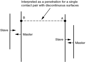
Figure 38.1.2–1 shows an example with a large, unintended initial overclosure. In this case a single contact pair with discontinuous surfaces is meant to enforce contact in two distinct regions (Table 35.3.1–1 “Orientation considerations for shell-like surfaces” in “Defining contact pairs in Abaqus/Standard,” Section 35.3.1, shows which contact formulations allow discontinuous surfaces). The arrows in Figure 38.1.2–1 show the positive normal direction for each surface region. The surface-to-surface contact formulation searches along the slave-surface normal direction (in the positive and negative directions) for potential interaction points on the master surface. The search emanating from point A identifies point B as the only potential interaction point for point A in this example. The contact pair interprets this as a valid penetration because no better candidate interaction location is found and surface normals are opposed at points A and B. Methods to avoid this unintended overclosure include:
defining separate contact pairs with continuous surfaces for each of the two distinct contact regions; and
specifying general contact, which filters out nearly all unintended initial overclosures.
The cause of unintended initial overclosures may be less obvious for three-dimensional models with complex surfaces. The most important step in overcoming this problem is identifying which regions of respective surfaces are involved in an unintended initial overclosure. For a surface-to-surface contact pair without strain-free adjustments, a portion of the master surface should be apparent behind the slave surface (opposite the slave surface normal direction) at a distance consistent with the reported (negative) COPEN value. For a node-to-surface contact pair, the direction to the interaction point on the master surface typically corresponds to a local minimum distance between the slave and master surfaces.
As previously discussed, Abaqus/Standard optionally interprets initial overclosures as interference fits. You should use one of the methods discussed above to remove any initial overclosures that are an unintended result of mesh discretization or errors in defining contact surfaces. In some cases the interference fit may be intended but may be too large to be resolved robustly with the method that is used by default for contact pairs in Abaqus/Standard (which is to resolve overclosures in a single increment). In this situation you should modify the contact model to allow resolution of overclosures over multiple increments (see “Modeling contact interference fits in Abaqus/Standard,” Section 35.3.4, for more information). If you choose to have initial overclosures treated as interference fits for general contact, they are automatically resolved over multiple increments (see “Controlling initial contact status in Abaqus/Standard,” Section 35.2.4).
Rigid body motion is generally not a problem in dynamic analysis. In static problems rigid body motion occurs when a body is not sufficiently restrained. “Numerical singularity” warning messages and very large displacements indicate unconstrained motion in a static analysis. Therefore, if contact is used to constrain rigid body motion in static problems, ensure that the appropriate surface pairs are initially in contact (see “Controlling initial contact status in Abaqus/Standard,” Section 35.2.4, and “Adjusting initial surface positions and specifying initial clearances in Abaqus/Standard contact pairs,” Section 35.3.5). If necessary, define the model geometry to give a small initial overclosure to the contact pair, or use boundary conditions to move the structures into contact in the first step. The boundary conditions, which are unnecessary in subsequent steps, can be removed after the body is adequately constrained through contact with other components. Similarly, if a rigid body is meant to translate only, constrain its rotational degrees of freedom.
Frictional sticking can constrain rigid body motion. However, contact pressure must develop before friction can be generated. Therefore, friction is not effective in constraining rigid body motion when surfaces first come into contact. You must temporarily eliminate rigid body motion by defining a boundary condition or by grounding the body with soft springs or dashpots.
If you are unable to prevent rigid body motion through modeling techniques, Abaqus/Standard offers some tools to automatically stabilize rigid bodies in contact simulations. These tools are discussed in “Automatic stabilization of rigid body motions in contact problems” in “Adjusting contact controls in Abaqus/Standard,” Section 35.3.6.
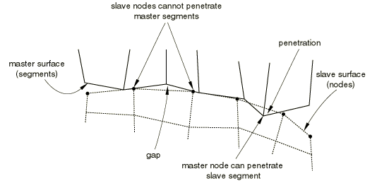
Over the course of an analysis, you may notice undesirable behavior between contact surfaces (excessive penetration, unexpected openings, inaccurate application of forces, etc.). This behavior often results in nonconvergence and termination of an analysis. These problems can arise from a number of causes related to mesh, element selection, and surface geometry.
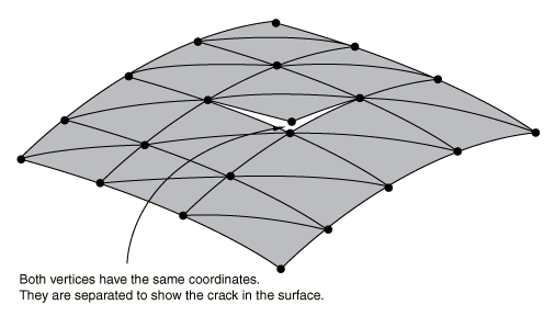
When defining three-dimensional surfaces for use in finite-sliding applications, avoid defining two surface nodes with the same coordinates. Such a definition can give rise to a seam, or crack, in the surface as shown in Figure 38.1.2–2.
If viewed with the default plotting options in Abaqus/CAE, this surface will appear to be a valid, continuous surface; however, if this surface is used as the master surface for finite-sliding, node-to-surface contact, a slave node sliding along the surface may fall through this crack and get “stuck” behind the master surface. Similar problems can occur for finite-sliding, surface-to-surface contact. Typically, convergence problems will result that may cause Abaqus/Standard to terminate the analysis.Use the edge display options in the Visualization module of Abaqus/CAE to identify any unwanted cracks in the surfaces used in the model. The cracks will appear as extra perimeter lines in the interior of the surface. Duplicate nodes can be avoided easily by equivalencing nodes when creating the model in a preprocessor.
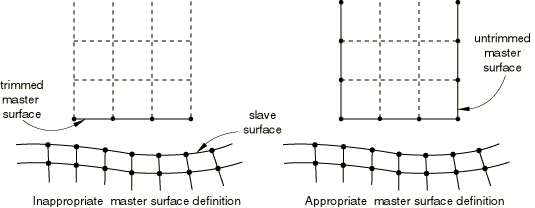
When modeling finite-sliding contact, ensure that the master surface definition extends far enough to account for all expected motions of the contacting parts. Contact along the perimeter of master surfaces should be avoided with the node-to-surface contact formulation.. Abaqus/Standard assumes that the mating slave surface nodes can fall off the free edge of the master surface, which can cause problems if a slave node wraps around and approaches its mating master surface from behind. Figure 38.1.2–3 illustrates appropriate and inappropriate master surface definitions.
A slave node that falls off a master surface in one iteration may find itself contacting the surface in the very next iteration; this phenomenon is known as chattering. If chattering continues, Abaqus/Standard may not be able to find a solution. This problem is less likely with the surface-to-surface formulation approach, because each contact constraint is based on a region of the slave surface rather than individual slave nodes. Request detailed contact printout to the message (.msg) file to monitor the history of a slave node that might slide off the master surface (see “The Abaqus/Standard message file” in “Output,” Section 4.1.1). The message file output will show the cyclic opening and closing of contact at a slave node, which will indicate where the master surface needs to be modified.For node-to-surface contact you can extend the master surface beyond the perimeter of the physical body that it approximates to avoid chattering problems. Chattering can also occur with some contact elements, such as slide line and rigid surface contact elements. Slide line contact elements can also be extended. See “Extending master surfaces and slide lines,” Section 35.3.8, for details.
Falling off the edge of a master surface in small-sliding contact problems is not an issue since slave nodes do not slide on the actual surface of the model. Instead, each slave node interacts with a flat, infinite contact plane. This plane is associated with the set of master surface nodes that are closest to the slave node in the undeformed configuration. For details about small-sliding contact, see “Contact formulations in Abaqus/Standard,” Section 37.1.1.
Several problems are caused by surfaces created on very coarse meshes. Some of these problems depend on your choice of contact discretization, as discussed later in “Discrepancies between contact formulations.”
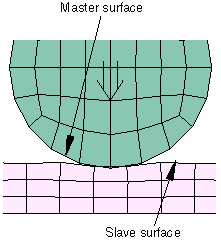
When a coarsely meshed surface is used as a slave surface for node-to-surface contact, the master surface nodes can grossly penetrate the slave surface without resistance (see Figure 38.1.2–4). This situation is common when nonmatching meshes come into contact. Refining the slave surface tends to alleviate this problem.
Figure 38.1.2–4 Master surface penetrations into the slave surface due to a coarse mesh of the slave surface for node-to-surface contact.
Surface-to-surface contact will generally resist penetrations of master nodes into a coarse slave surface; however, this formulation can add significant computational expense if the slave mesh is significantly coarser than the master mesh (see “Contact formulations in Abaqus/Standard,” Section 37.1.1, for further discussion).
If the mesh on a surface is too coarse, it is possible for a contact interaction to occur entirely within the bounds of a single element. This typically happens when the two contacting surfaces have dissimilar curvature, as depicted in Figure 38.1.2–5.
The results from such an interaction are unreliable and generally unrealistic. If the model in Figure 38.1.2–5 uses node-to-surface contact, the master surface penetrates the slave surface without resistance until it encounters a slave node, as discussed above. If the master and slave designations are reversed, the contact constraint is applied at a single slave node; this concentration creates inaccurately high calculations of the contact pressure. If the model uses surface-to-surface contact, excessive penetration is not likely to occur. However, with only a small number of constraint points involved in the interaction, the averaging algorithm used to enforce surface-to-surface contact performs poorly. Inaccurate contact stress and pressure calculations result.If contact is occurring at a single element, refine the mesh to spread the interaction across multiple element faces.
Coarsely meshed, curved master surfaces in small-sliding simulations can lead to unacceptable solution accuracy due to the approximate nature of the “master planes.” Using a more refined mesh to define the master surface will improve the overall accuracy of the solution in small-sliding problems. However, unless perfectly matching meshes are used, local oscillations in the contact stress may still be observed, even in refined models.
Inaccurate local results may occur if second-order heat transfer elements are used to model a thermal interface and the meshes do not match across the surfaces. The worst results will be obtained when the midside node of an element on one surface is closest to the corner node of an element on the other surface. If a nonmatching mesh must be used in the model, use first-order elements or use a more refined mesh.
Second-order elements not only provide higher accuracy but also capture stress concentrations more effectively and are better for modeling geometric features than first-order elements. Surfaces based on second-order element types work well with the surface-to-surface contact formulation but, in some cases, do not work well with the node-to-surface formulation (see “Contact formulations in Abaqus/Standard,” Section 37.1.1, for a discussion of these contact formulations).
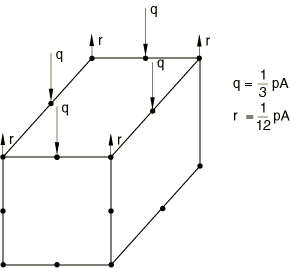
Some second-order element types are not well-suited for underlying the slave surface with the combination of a node-to-surface contact formulation and strict enforcement of “hard” contact conditions, because of the distribution of equivalent nodal forces when a pressure acts on the face of the element. As shown in Figure 38.1.2–6, a constant pressure applied to the face of a second-order element without a midface node produces forces at the corner nodes acting in the opposite sense of the pressure.
Figure 38.1.2–6 Equivalent nodal loads produced by a constant pressure on the second-order element face in “hard” contact simulations.
The element families C3D20(RH), C3D15(H), S8R5, and M3D8 are converted to the families C3D27(RH), C3D15V(H), S9R5, and M3D9, respectively. Since Abaqus/Standard does not convert second-order coupled temperature-displacement, coupled thermal-electrical-structural, and coupled pore pressure–displacement elements, you should specify a penalty or augmented Lagrange constraint enforcement method to approximate hard pressure-overclosure behavior (see “Contact constraint enforcement methods in Abaqus/Standard,” Section 37.1.2). Abaqus/Standard will interpolate nodal quantities, such as temperature and field variables, at the automatically generated midface nodes when values are prescribed at any of the user-defined nodes.
Second-order tetrahedral elements (C3D10 and C3D10I) have zero contact force at their corner nodes. This combination of second-order triangular slave facets, a node-to-surface contact formulation, and strict enforcement of “hard” contact conditions is disallowed to avoid a high likelihood of convergence problems and poor predictions of contact pressures that would occur with this combination. To avoid this combination, use at least one of the following alternatives:
Use the surface-to-surface contact formulation (generally recommended) instead of the node-to-surface contact formulation;
Use the penalty constraint enforcement method (generally recommended) or augmented Lagrange constraint enforcement method instead of strict enforcement of “hard” contact conditions; or
Use modified 10-node tetrahedral elements (C3D10M) instead of second-order tetrahedral elements.
Abaqus/Standard offers a number of methods to adjust the solver iteration scheme, sometimes resulting in a more efficient analysis with a minimal effect on accuracy.
By default, Abaqus/Standard continues to iterate until the severe discontinuities associated with changes in contact status are sufficiently small (or no severe discontinuities occur) and the equilibrium (flux) tolerances are satisfied. Alternatively, you can choose a different approach in which Abaqus/Standard continues to iterate until no severe discontinuities occur. These two approaches are discussed in more detail in “Severe discontinuities in Abaqus/Standard” in “Defining an analysis,” Section 6.1.2. The default treatment of severe discontinuity iterations reduces the likelihood of excessive iterations associated with chattering between contact states when the contact conditions are weakly determined. An example of a region with weakly determined contact conditions is near the center of a flat punch that contacts a thin plate supported at its edges.
For most types of contact, if during an iteration the penetration calculated for any contact pair exceeds a specific distance (![]() ), Abaqus/Standard abandons the increment and tries again with a smaller increment size. There is no critical penetration distance for finite-sliding, surface-to-surface contact (including general contact) and for small-sliding contact in geometrically linear analyses.
), Abaqus/Standard abandons the increment and tries again with a smaller increment size. There is no critical penetration distance for finite-sliding, surface-to-surface contact (including general contact) and for small-sliding contact in geometrically linear analyses.
The default value of ![]() is the radius of a sphere that circumscribes a characteristic surface element face. When calculating the default value, Abaqus/Standard uses only the slave surface of the contact pair. The value of
is the radius of a sphere that circumscribes a characteristic surface element face. When calculating the default value, Abaqus/Standard uses only the slave surface of the contact pair. The value of ![]() for each contact pair in the model is printed in the data (.dat) file. While the default value of
for each contact pair in the model is printed in the data (.dat) file. While the default value of ![]() should prove to be sufficient for the majority of contact simulations, in some cases it may be necessary to change the default value for a given contact pair. These cases include:
should prove to be sufficient for the majority of contact simulations, in some cases it may be necessary to change the default value for a given contact pair. These cases include:
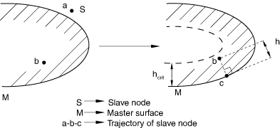
Models in which the master surface is highly curved. The default value of ![]() may sometimes lead to situations as shown in Figure 38.1.2–7. During the iterative solution process a slave node initially at point a may move to point b, penetrating the master surface with overclosure h less than
may sometimes lead to situations as shown in Figure 38.1.2–7. During the iterative solution process a slave node initially at point a may move to point b, penetrating the master surface with overclosure h less than ![]() . Abaqus/Standard may attempt to move the slave node to point c on the master surface. To avoid this situation, specify a smaller value for
. Abaqus/Standard may attempt to move the slave node to point c on the master surface. To avoid this situation, specify a smaller value for ![]() to force Abaqus/Standard to abandon the increment and to try a smaller increment size.
to force Abaqus/Standard to abandon the increment and to try a smaller increment size.
Models in which Abaqus/Standard cannot calculate a reasonable ![]() because a node-based surface is used. If there are other contact pairs in the model with surfaces, Abaqus/Standard uses the average dimension of all of the slave surface element faces. If there are no other contact pairs, Abaqus/Standard uses a characteristic element dimension of the entire model.
because a node-based surface is used. If there are other contact pairs in the model with surfaces, Abaqus/Standard uses the average dimension of all of the slave surface element faces. If there are no other contact pairs, Abaqus/Standard uses a characteristic element dimension of the entire model.
Models in which the contact face dimensions in a slave surface vary greatly.
Models in which the slave surface mesh is very refined compared with the typical surface dimensions so that overclosures much larger than the default ![]() can be resolved easily.
can be resolved easily.
Models in which contact pairs with softened contact allow significant penetration (see “Contact pressure-overclosure relationships,” Section 36.1.2).
| Input File Usage: | *CONTACT PAIR, HCRIT= |
| Abaqus/CAE Usage: | You cannot adjust the default value of |
Although an analysis involving contact runs to completion, the results may seem unrealistic. This is sometimes due to modeling errors and sometimes due to the specialized output format of certain contact formulations. In addition to degrading contact output, the factors discussed below also tend to degrade convergence behavior, so avoiding these factors may improve convergence behavior.
Nonuniform contact pressure distributions are likely to occur when very different mesh densities are used on the two deformable surfaces making up a contact interaction. The nonuniformity can be particularly pronounced when “hard” contact is modeled and both surfaces are modeled with second-order elements, including modified, second-order tetrahedral elements. In such cases oscillations and “spikes” in the contact pressure may occur. Smoother contact pressures may be obtained for surfaces modeled with second-order elements by using penalty-type contact constraint enforcement (see “Contact constraint enforcement methods in Abaqus/Standard,” Section 37.1.2).
For second-order axisymmetric elements the contact area is zero at a node lying on the symmetry axis ![]() . To avoid numerical singularity problems caused by a zero contact area, Abaqus/Standard calculates the contact area as if the node were a small distance from the symmetry axis. This may result in inaccurate local contact stresses calculated for nodes located on the symmetry axis.
. To avoid numerical singularity problems caused by a zero contact area, Abaqus/Standard calculates the contact area as if the node were a small distance from the symmetry axis. This may result in inaccurate local contact stresses calculated for nodes located on the symmetry axis.
Contact of a surface with itself (self-contact) is provided for cases in which the original geometry is very different from the (deformed) geometry at which contact takes place. It would then be difficult for you to predict which parts of the surface will come into contact with each other. Where possible, it is always computationally more economical to declare parts of the surface as master and parts as slave. The same unpredictability makes it impossible to determine a priori which side will be the master and which side the slave. Therefore, Abaqus/Standard uses a symmetric contact model: every single node of the surface can be a slave node and can simultaneously belong to master segments with respect to all other nodes.
Because each surface is acting as both a slave and a master, the results of symmetric contact analyses can be confusing and inconsistent. These difficulties are discussed more fully in “Using symmetric master-slave contact pairs to improve contact modeling” in “Defining contact pairs in Abaqus/Standard,” Section 35.3.1.
The term overconstraint refers to a situation in which multiple kinematic constraints outnumber the degrees of freedom on which they act. Overconstraints often lead to inaccurate solutions or failure to obtain a converged solution. Contact conditions strictly enforced with the direct constraint enforcement method (using Lagrange multipliers) are sometimes involved in overconstraints. See “Overconstraint checks,” Section 34.6.1, for a detailed discussion and examples of overconstraints and how Abaqus/Standard will treat overconstraints based on the following classifications:
Overconstraints detected in the model preprocessor
Overconstraints detected and resolved during analysis
Overconstraints detected in the equation solver
Contact conditions with a softened behavior or enforced with the penalty or augmented Lagrange method will not combine with other constraints to cause “strict overconstraints”; however, “softened overconstraints” can:
cause zero pivots or ill-conditioning in the equation solver if the stiffness contributions associated with contact are many orders of magnitude higher than the stiffness contributions from typical elements;
prevent a tight penetration tolerance from being achieved with the augmented Lagrange method; and
cause oscillations in contact stress solutions, particularly if the contact stiffness is high.
If nodes in a contact pair are overconstrained but the equation solver does find a solution, the contact forces become indeterminate and may become excessively high, particularly in tied contact pairs. Check the time average force (or moment, or flux) reported in the message file, or use Abaqus/CAE to view the diagnostic information interactively (for more information, see Chapter 41, “Viewing diagnostic output,” of the Abaqus/CAE User's Manual). If it is many orders of magnitude larger than the residual forces (or moments, or fluxes), an overconstraint may have occurred, and there is no guarantee that Abaqus/Standard has found the correct solution. Another sign that the model is overconstrained is that the analysis begins to converge in a single iteration in every increment when the nonlinearities should require at least several iterations. Overconstraints should be avoided only by changing the contact definition or other constraint type involved.
Automatic resolution of contact overconstraints sometimes depends on whether two contact pairs refer to the same surface interaction definition. For example, consider a case in which two contact pairs have a common master surface and share some slave nodes (perhaps along a common edge of two slave surfaces). Overconstraints will occur at the common slave nodes if the two contact pairs refer to different surface interaction definitions (even if the surface interactions are equivalent); however, Abaqus/Standard automatically avoids these overconstraints if the two contact pairs refer to the same surface interaction definition. (See “Assigning contact properties for contact pairs in Abaqus/Standard,” Section 35.3.3, for a discussion of how to assign surface interaction definitions to contact pairs.)
The different contact formulations available in Abaqus/Standard (see “Contact formulations in Abaqus/Standard,” Section 37.1.1) allow for a great deal of flexibility when modeling contact simulations. However, two nearly identical simulations that differ only in the contact formulation being used will sometimes generate varying results. This is primarily because of the different ways that contact formulations interpret contact conditions. Certain formulations are better suited to particular situations.
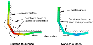
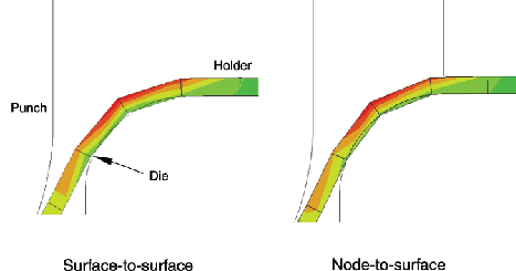
The most observable difference between node-to-surface and surface-to-surface discretization is the amount of penetration that occurs between surfaces. This is because node-to-surface discretization computes penetrations only at slave nodes, while surface-to-surface discretization computes penetrations in an average sense over a finite region. For example, when a slave surface slides across a convex portion of a master surface, the slave surface will tend to ride a bit higher with surface-to-surface discretization than with node-to-surface discretization, as shown in Figure 38.1.2–8 (the opposite is true at a concave portion of a master surface). Figure 38.1.2–9 shows another case in which the two contact discretizations behave fundamentally differently due to the different approaches to computing penetrations. Both discretizations converge to the same behavior as the mesh is refined.
Figure 38.1.2–8 Comparison of contact discretizations in an example with convex curvature in the master surface (forming application).
The differences in computed penetrations can sometimes fundamentally affect the results of an analysis. Be aware of this possibility when converting models from one contact formulation to another. Various aspects of preexisting models, such as the friction coefficient or the pressure-overclosure relationship, may have been inadvertently “tuned” to the behavior that occurs with a particular contact formulation.
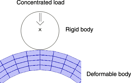
Figure 38.1.2–10 shows an example in which a circular rigid body is pushed into a deformable body.
In the initial configuration shown, the two bodies touch at a single point, which corresponds to a slave node location. The following scenarios are likely for respective analyses of this model with node-to-surface and surface-to-surface discretization:With node-to-surface discretization, the first iteration is performed with one active contact constraint. A converged solution is obtained with a reasonable number of iterations and increments.
With surface-to-surface discretization, penetrations are computed in an average sense over finite regions of the surface, so a positive gap distance is computed for all potential contact constraints even though the surfaces touch at one of the slave nodes. However, the finite-sliding, surface-to-surface contact formulation detects that the surfaces are initially touching and by default automatically activates localized contact damping in the neighborhood where the gap distance is zero. Without such damping, Abaqus/Standard may not obtain a converged solution due to an unconstrained rigid body mode. This contact damping typically has an insignificant effect on the converged solution, and the damping is completely removed by the end of the step.
| Input File Usage: | Use the following option to deactivate automatic localized contact damping at artificial surface gaps for contact pair definitions: |
*CONTACT PAIR, MINIMUM DISTANCE=NO Use the following option to deactivate automatic localized contact damping at artificial surface gaps for general contact definitions: *CONTACT INITIALIZATION DATA, MINIMUM DISTANCE=NO |
| Abaqus/CAE Usage: | You cannot deactivate automatic localized contact damping at artificial surface gaps in Abaqus/CAE. |
Node-to-surface discretization uses a contact normal direction based on the master surface normal, whereas surface-to-surface discretization uses a contact normal direction based on the slave surface normal (averaged over a region nearby the slave node). For most active contact definitions the slave and master surfaces are nearly parallel, so the master and slave normals are approximately aligned; in which case this distinction in how the contact normal is determined is not significant. However, in some cases the differences in the contact normal can be significant.
When modeling large interference fits, surface-to-surface discretization can sometimes cause tangential motion of the slave surface as the overclosures are resolved. This tangential motion may have undesirable effects on an analysis. See “Controlling initial contact status in Abaqus/Standard,” Section 35.2.4, and “Modeling contact interference fits in Abaqus/Standard,” Section 35.3.4, for more details.
Contact constraints involving geometric edges of surfaces sometimes use a significantly different contact normal depending on which contact discretization approach is used, because the normals for the slave and master surfaces may not directly oppose each other.
The contact opening distance output variable (COPEN) can vary considerably depending on what type of contact formulation is used if the contact surfaces are not parallel. For node-to-surface discretization, the opening distance that is reported approximates the closest distance to the master surface; for surface-to-surface discretization, the opening distance that is reported corresponds to the distance from the slave surface to the master surface along the slave normal direction. The opening distance for surface-to-surface discretization is undefined if a line emanating from the slave surface in the slave normal direction does not intersect the master surface (as discussed in “Using the small-sliding tracking approach” in “Contact formulations in Abaqus/Standard,” Section 37.1.1, if a small-sliding constraint cannot be formed in such a case for the small-sliding, surface-to-surface formulation, Abaqus/Standard automatically reverts to the node-to-surface approach for individual constraints).
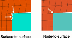
The finite-sliding, surface-to-surface formulation is often better-suited than other contact formulations for modeling contact near corners. In the example shown in Figure 38.1.2–11, the slave surface is on the “outer” body (i.e., the body with a reentrant corner). With node-to-surface discretization a single constraint acts at the corner slave node in the “average” normal direction of the master surface, which often leads to poor resolution of contact, non-physical response, and even early termination of an analysis. However, surface-to-surface discretization generates two constraints near the corner for the respective faces, as shown in Figure 38.1.2–11, resulting in more stable contact behavior.