35.4.2 Midsurface modeling of a complex part

This example uses several techniques and tools to create the midsurface model for a reinforced structural component.

The solid model

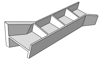
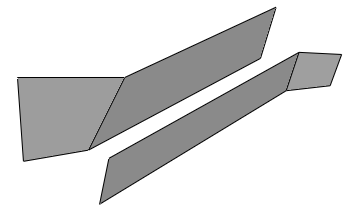
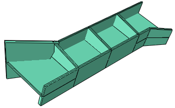
The model in this example is the structural beam shown in Figure 35–11. The reinforcing ribs, different thicknesses, and asymmetrical shape of the beam do not allow for a simple beam section representation. The complexity of the part combined with its thin cross-sections make it a good candidate for replacement with a midsurface model. As in the previous example, bending performance will be improved by using a shell model for the mesh instead of thin solid sections.

Figure 35–11 The solid model of the reinforced beam.

Assign the midsurface region

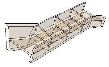
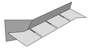
Use the Assign Midsurface Region tool in the Part module to remove geometry from the active representation of the beam and to create a reference representation of the original solid geometry, as shown in Figure 35–12.

Figure 35–12 The reference representation of the beam.

The reference representation is an abstract representation of the original part. It retains the original geometry of the part, but it cannot be used in the analysis. The reference representation appears by default in the Part module; you can toggle it off and on using the Show Reference Representation tool

located with the visible object tools in the main toolbar. For more information, see “Understanding the reference representation,” Section 35.2, and “Assigning a midsurface region,” Section 35.5.1.

Create the shell representation

You must create a shell representation of the beam that can be analyzed by Abaqus. Creating a shell for this part requires multiple steps and tools. There may be several equally valid ways to produce an accurate shell representation for a model. The following steps use tools from the Geometry Edit toolset to create the new shell faces.

Use the offset face tool to create shell faces for the vertical upper left side of the beam.
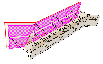
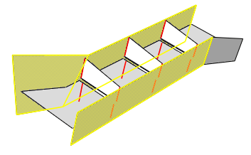
Select faces from the reference representation to create the offset shell. Use Auto Select to select the target faces. The faces to offset and the target faces are shown in red and magenta, respectively, in Figure 35–13.
Figure 35–13 Selected faces to create the offset for the upper left side.
The faces to offset are the two outer vertical faces toward the rear. The target faces are the nine faces, mostly unconnected, that comprise the inner surface of the same beam wall. The Fraction distance to closest point on face method is used with an entry of 0.5 to create the offset with half the thickness of the thinner main portion along the top of the beam. Using this option prevents the thicker sections at the left and along the bottom of the beam from creating an offset larger than the thinner portion. The Auto trim to reference representation option is used for this step. This operation extends the faces during the offset process and then trims them along the edges of the reference representation. Auto trim may fail when multiple offset and target faces are selected; if auto trim fails, Abaqus/CAE displays a warning indicating the failure. You can use the extend faces tool to extend the new faces to meet the edges of the reference representation. The resulting offset faces are shown in Figure 35–14.
Figure 35–14 The resulting offset faces.
Repeat the process from Step 1 to create offset faces for the opposite side of the beam.
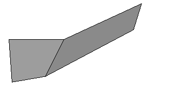
The resulting shell model now contains the two outer surfaces of the beam, as shown in Figure 35–15.
Figure 35–15 The offset faces from the first and second steps.
Create offset faces for the four horizontal sections that connect the two side walls.
You can create the faces in a single offset operation by selecting the four top faces to offset and using Auto Select to select the corresponding bottom faces. In this case Auto trim to reference representation is toggled off, so the new faces are not extended and trimmed. The shell model of the horizontal faces is shown in Figure 35–16. (The faces created in Step 2 have been suppressed for clarity.) Notice the gaps between the horizontal faces where they meet the vertical reinforcement ribs in the original part. Similar gaps exist between the horizontal shell faces and the side walls created in the previous two steps.
Figure 35–16 The horizontal offset faces.
Repeat the process from Step 3 to create offset faces for the vertical ribs that connect the sides of the beam.
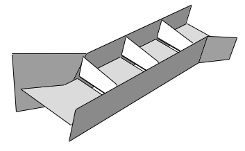
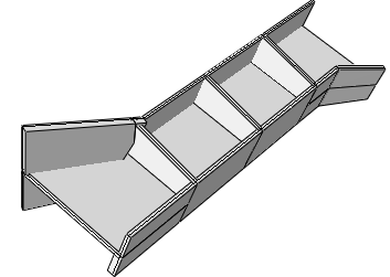
The midsurface shell model now contains faces representing nearly all of the solid geometry, as shown in Figure 35–17. However, there are gaps between most of the faces due to the thickness of the original solid structure.
Figure 35–17 The midsurface model with gaps between the faces.
Close the gaps between the vertical ribs and the beam sides.
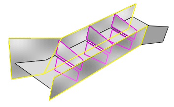
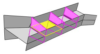
Use the extend faces tool to extend the six vertical ribs to intersect with the sides. The selected faces and target faces are shown in magenta and yellow, respectively, in Figure 35–18.
Figure 35–18 Specifying the faces to extend and the target faces.
When you click OK, Abaqus/CAE updates the highlighting to indicate the edges along which the faces will be extended, as shown in Figure 35–19, and displays a warning dialog box with options allowing you to accept the selection, to extend all edges of the selected faces, or to cancel the extend faces procedure.
Figure 35–19 The edges where the vertical faces will be extended.
Use the extend faces tool to extend the horizontal faces to intersect with the sides of the beam.
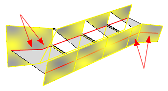
In this case, use the Specify edges of faces to extend method with Up to target faces to pick the edges and faces, respectively, shown in Figure 35–20. When Abaqus/CAE highlights the edges indicating the areas that will be extended, the four edges indicated by arrows in the figure are removed from the selection because they do not completely match the target faces. Click No to use the previous selection of edges.
Figure 35–20 The edges along which the horizontal faces will be the extended.
Close the remaining gaps between the horizontal and vertical connecting sections of the beam. You can use either the blend faces tool or the extend faces tool to complete the midsurface model by closing the remaining gaps between the horizontal and vertical connecting sections of the beam.
1. Use the extend faces tool with the selections shown in Figure 35–21.
  Toggle on Trim to extended underlying target surfaces so that Abaqus/CAE will extend and trim the vertical faces to their implied intersections with the selected target face.
  Figure 35–21 Filling the gaps between the vertical reinforcing ribs.
2. Use the blend faces tool to fill the remaining gaps.
  The tool must be used three times to fill the three remaining gaps in the model.

Assign thicknesses

All the original solid geometry has now been replaced with shell geometry. To complete the model, you should verify that the shells have appropriate thickness information. Click the assign thickness and offset tool . Abaqus/CAE highlights any shell faces that do not have thickness data. In this case, since the shell faces were all created using the offset, extend, and blend tools, all of the faces already have thickness data assigned. If there were faces without thickness data, you would select each face and, using the Compute thickness from opposite faces method in the Assign thickness and Offset dialog box, pick appropriate top and bottom faces from the reference representation to create the missing thicknesses.

To view the model with shell thicknesses, you can toggle on Render shell thickness in the Part Display Options dialog box (for more information, see “Visualizing shell thicknesses,” Section 35.5.3). As shown in Figure 35–22, the resulting view includes the variations in thickness that were in the original solid model.

Figure 35–22 Shell faces with thickness displayed.

Assign a shell section

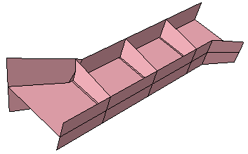
Use the Property module to create a shell section and assign it to the midsurface model. When you create the shell section, you can enter an arbitrary value for the shell thickness. When you subsequently assign the section to the shell, you specify that the thickness and the shell offset are calculated from the geometry in the Edit Section Assignment dialog box. Abaqus/CAE ignores the thickness value that you entered for the shell section and uses the thicknesses assigned to the faces in the Part module. For more information, see “Assigning a section,” Section 12.15.1. Figure 35–23 shows the completed midsurface model with section thicknesses after section assignment in the Property module. The geometry is identical to that in Figure 35–22.

Figure 35–23 The completed midsurface geometry with shell thicknesses.

Mesh the part

Abaqus/CAE colors the shell part pink in the Mesh module to indicate it can be meshed using the free meshing technique, as shown in Figure 35–24.

Figure 35–24 Free meshing can be applied to the part.

Before seeding and meshing the part, you can apply automatic virtual topology to remove small details that are not needed in the mesh (for more information, see “Creating virtual topology automatically,” Section 75.6.1). The default automatic virtual topology settings should remove the blended face edges and other small details that would unnecessarily constrain the part mesh.

Note: Automatic virtual topology may fail if neighboring faces have inconsistent normals. If this occurs, return to the Part module and use the tool in the Geometry Edit toolset to repair the face normals.

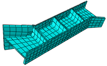
Apply default seeding and mesh controls, and generate the mesh on the part. The resulting mesh is shown in Figure 35–25, with the shell thickness displayed.

Figure 35–25 The resulting mesh with shell thickness rendering.