This simulation of the forming of a channel in a long metal sheet illustrates the use of rigid surfaces and some of the more complex techniques often required for a successful contact analysis in Abaqus/Standard.
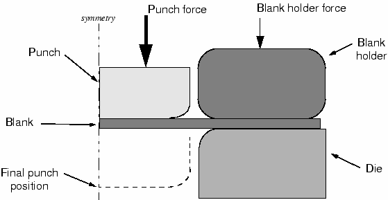
The problem consists of a strip of deformable material, called the blank, and the tools—the punch, die, and blank holder—that contact the blank. The tools are modeled as (analytical) rigid surfaces because they are much stiffer than the blank. Figure 12–15 shows the basic arrangement of the components.
The blank is 1 mm thick and is squeezed between the blank holder and the die. The blank holder force is 440 kN. This force, in conjunction with the friction between the blank and blank holder and the blank and die, controls how the blank material is drawn into the die during the forming process. You have been asked to determine the forces acting on the punch during the forming process. You also must assess how well the channel is formed with these particular settings for the blank holder force and the coefficient of friction between the tools and blank.A two-dimensional, plane strain model will be used. The assumption that there is no strain in the out-of-plane direction of the model is valid if the structure is long in this direction. Only half of the channel needs to be modeled because the forming process is symmetric about a plane along the center of the channel.
The model will use contact pairs rather than general contact, since general contact is not available for analytical rigid surfaces in Abaqus/Standard.
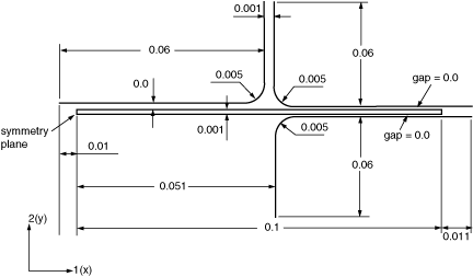
The dimensions of the various components are shown in Figure 12–16.
Two-dimensional, plane strain models are defined, by default, in the global 1–2 plane as shown in Figure 12–16. For the forming simulation, place the origin of this plane at the bottom left-hand corner of the blank (Figure 12–16). The 1-direction will be normal to the symmetry plane, which is located at ![]() .
.
The mesh for this simulation can be divided into the deformable blank and the rigid tools.
Blank
Once again, the element type should be selected before the mesh is designed. The mesh used for the blank should consist of four rows of 100 CPE4R elements (see Figure 12–17). Four rows of elements are used so that better resolution of the deformation through the thickness of the blank will be obtained.
The node and element numbers for the mesh shown in Figure 12–18 are from the model of this problem given in “Forming a channel with Abaqus/Standard,” Section A.13. These node and element numbers are used in the discussion that follows.
Tools
The tools are modeled with analytical rigid surfaces.
The steps that follow assume that you have access to the full input file for this example. This input file, channel.inp, is provided in “Forming a channel with Abaqus/Standard,” Section A.13. Instructions on how to fetch and run the script are given in Appendix A, “Example Files.” If you wish to create the entire model using Abaqus/CAE, please refer to “Abaqus/Standard 2D example: forming a channel,” Section 12.6 of Getting Started with Abaqus: Interactive Edition.
We first review the model definition, including the node and element definitions, and section and material properties.
Model description
The input file starts with a relevant description of the simulation and model in the *HEADING option.
*HEADING
Analysis of the forming of a channel
SI units (N, kg, m, s)
Nodal coordinates and element connectivity
Check that the preprocessor used the correct element type for the blank. Provide a meaningful element set name, such as BLANK, for the elements. The *ELEMENT option in this model follows:
*ELEMENT, TYPE=CPE4R, ELSET=BLANK
The model definition also specifies the creation of node sets so that parts of the model can be constrained and moved easily. These nodes are located on the centerline of the blank and have symmetric constraints into a node set called CENTER.
*NSET, NSET=CENTER
1,102,203,304,405
The node along the middle of the sheet at the left-hand side of the model, underneath the punch, is included in node set MIDLEFT.
*NSET, NSET=MIDLEFT
203,
Again, the node numbers in these option blocks are for the model in Figure 12–18; your node numbers may be different.
Two element sets, BLANK_B and BLANK_T, will be defined that contain the lower and upper rows of elements in the blank. These will be used to define the contact surfaces on the blank.
*ELSET, ELSET=BLANK_B, GENERATE
1,100,1
*ELSET, ELSET=BLANK_T, GENERATE
301,400,1
Section and material properties for the blank
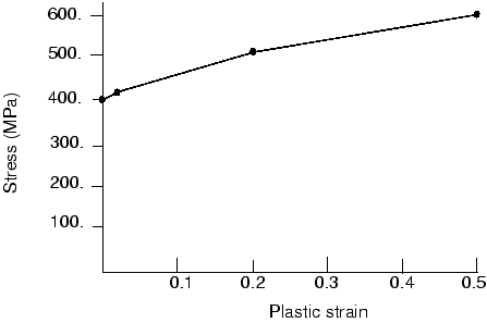
The blank is made from a high-strength steel (elastic modulus of 210.0 GPa, ![]() = 0.3). Its stress-strain behavior is shown in Figure 12–19. The material undergoes considerable work hardening as it deforms plastically. It is likely that plastic strains will be large in this analysis; therefore, hardening data are provided up to 50% plastic strain.
= 0.3). Its stress-strain behavior is shown in Figure 12–19. The material undergoes considerable work hardening as it deforms plastically. It is likely that plastic strains will be large in this analysis; therefore, hardening data are provided up to 50% plastic strain.
The blank is going to undergo significant rotation as it deforms. Reporting the values of stress and strain in a coordinate system that rotates with the blank's motion will make it much easier to interpret the results. Therefore, an *ORIENTATION option should be used to create a coordinate system that is aligned initially with the global coordinate system but moves with the elements as they deform. The following input options are needed to define the blank's element and material properties:
*ORIENTATION, NAME=LOCAL
1.,0.,0., 0.,1.,0.
1, 0
*SOLID SECTION, MATERIAL=STEEL, ORIENTATION=LOCAL,
ELSET=BLANK, CONTROL=EC-1
*SECTION CONTROLS, NAME=EC-1, HOURGLASS=ENHANCED
*MATERIAL, NAME=STEEL
*ELASTIC
2.1E11,0.3
*PLASTIC
400.E6, 0.0E-2
420.E6, 2.0E-2
500.E6,20.0E-2
600.E6,50.0E-2
The contact definitions for each part of the model are discussed here.
Rigid surfaces
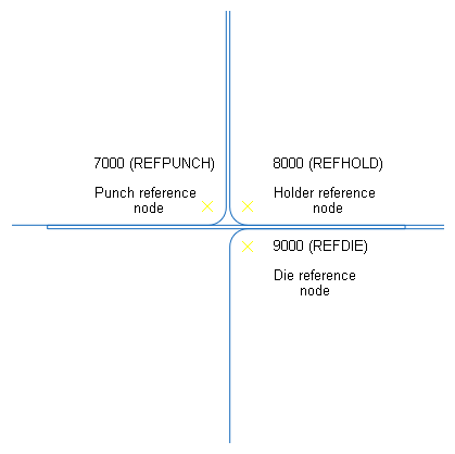
The blank holder, the punch, and the die are modeled with analytical rigid surfaces. A rigid body reference node will be assigned to each of these surfaces when they are created. If you did not create these rigid body reference nodes during preprocessing, add the following option block to your model:
*NODE, NSET=REFPUNCH
7000, 0.000, 0.06
*NODE, NSET=REFHOLD
8000, 0.1,0.06
*NODE, NSET=REFDIE
9000,0.1,-0.06
*NSET, NSET=NOUT
REFDIE, REFHOLD, REFPUNCH
Each node is placed in a node set to make the input file easy to read. While someone unfamiliar with the specific mesh used in the simulation may not know why boundary conditions are applied to node 7000, they might be able to guess why boundary conditions were applied to the REFPUNCH node. All reference nodes are also assigned to a set named NOUT to facilitate the history output requests that will follow.
To ensure that an analytical rigid surface's normals point toward the deformable surfaces that the rigid surface will contact, the segments composing the rigid surface must be defined in a particular order. For example, to create the correct normals for the surface PUNCH, define the surface from the top right corner to the bottom left corner of the punch. The following input to the model creates the surface PUNCH:
*SURFACE, TYPE=SEGMENTS, NAME=PUNCH, FILLET RADIUS=0.001
START,0.050, 0.060
LINE, 0.050, 0.006
CIRCL,0.045, 0.001, 0.045,0.006
LINE,-0.010, 0.001
*RIGID BODY, ANALYTICAL SURFACE=PUNCH, REF NODE=7000
The parameter TYPE=SEGMENTS specifies that a two-dimensional rigid surface is being defined. The NAME parameter specifies the name of the surface, PUNCH. The data lines define the geometry of the surface. The first data line always has the word “START” followed by the 1- and 2-coordinates of the starting point for the surface. The subsequent lines define line, circular, and parabolic segments. For this surface the second data line defines a straight line from the start position (0.05, 0.060) to (0.050, 0.006). The third data line defines a circular arc from the end of the straight line (0.05, 0.006) to (0.045, 0.001) with the center of the circle located at (0.045, 0.006). The last data line defines a straight line from the end of the arc to (0.010, 0.001).
This definition should produce a smooth rigid surface but, to be safe, the FILLET RADIUS parameter specifies that a 1 mm fillet radius should be used to smooth any discontinuities in the surface definition. It is always good practice to add the FILLET RADIUS parameter to the definition of any analytical rigid surface.
The *RIGID BODY option is used to bind the analytical surface to a rigid body with its rigid body reference node specified by the REF NODE parameter and the surface referred to by its name, using the ANALYTICAL SURFACE parameter.
The rigid surfaces for the blank holder and the die are defined in a similar way. The following option blocks define the surfaces on these tools:
*SURFACE, TYPE=SEGMENTS, NAME=HOLDER, FILLET RADIUS=0.001
START,0.110, 0.001
LINE, 0.056,0.001
CIRCL,0.051,0.006, 0.056,0.006
LINE, 0.051,0.060
*RIGID BODY, ANALYTICAL SURFACE=HOLDER, REF NODE=8000
**
*SURFACE, TYPE=SEGMENTS, NAME=DIE, FILLET RADIUS=0.001
START,0.051,-0.060
LINE, 0.051,-0.005
CIRCL,0.056,0.,0.056,-0.005
LINE, 0.11, 0.
*RIGID BODY, ANALYTICAL SURFACE=DIE, REF NODE=9000
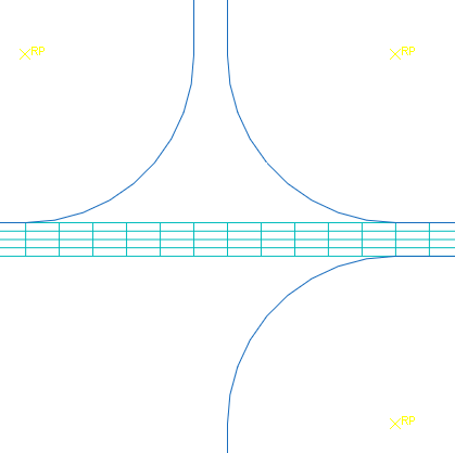
All of the rigid surfaces in this simulation extend beyond the deformable blank to ensure that there is no possibility that slave nodes will slide behind any of them. The initial configuration of these surfaces and the locations of their reference nodes are shown in Figure 12–20.
Deformable surfaces
Using the two element sets defined on the blank, create a contact surface on the top of the blank, called BLANK_T, and one on the bottom, called BLANK_B. If you use the automatic free surface generation capability, the option blocks will look like
*SURFACE, NAME=BLANK_B
BLANK_B,
*SURFACE, NAME=BLANK_T
BLANK_T,
Contact pairs
Contact must be defined between the top of the blank and the punch, the top of the blank and the blank holder, and the bottom of the blank and the die. The rigid surface must be the master surface in each of these contact pairs. Each contact pair must refer to a *SURFACE INTERACTION option that defines a surface interaction model governing how the surfaces of the contact pair interact with each other. Multiple contact pairs can refer to the same *SURFACE INTERACTION option.
In this example we assume that the friction coefficient is zero between the blank and the punch. The friction coefficient between the blank and the other two tools is assumed to be 0.1. Therefore, two *SURFACE INTERACTION options must be used in the model: one with friction and one without. Frictionless contact is the default in Abaqus, so no *FRICTION option is needed in the surface interaction definition for the contact pair.
The option blocks to define the contact pairs and surface interactions in your model will look like
*CONTACT PAIR, INTERACTION=FRIC, TYPE=SURFACE TO SURFACE
BLANK_B, DIE
BLANK_T, HOLDER
*CONTACT PAIR, INTERACTION=NOFRIC, TYPE=SURFACE TO SURFACE
BLANK_T, PUNCH
*SURFACE INTERACTION, NAME=FRIC
*FRICTION
0.1,
*SURFACE INTERACTION, NAME=NOFRIC
For each contact pair the surface-to-surface contact discretization technique has been used, which controls the location where contact constraints will be generated and enforced.
There are two major sources of difficulty in Abaqus/Standard contact analyses: rigid body motion of the components before contact conditions constrain them, and sudden changes in contact conditions, which lead to severe discontinuity iterations as Abaqus/Standard tries to establish the exact condition of all contact surfaces. Therefore, wherever possible, take precautions to avoid these situations.
Removing rigid body motion is not particularly difficult. Simply ensure that there are enough constraints to prevent all rigid body motions of all the components in the model. This approach may mean using boundary conditions initially to get the components into contact, instead of applying loads directly. Using this approach may require more steps than originally anticipated, but the solution of the problem should proceed more smoothly.
Alternatively, contact controls may be used to stabilize rigid body motion automatically. With this approach Abaqus/Standard applies viscous damping to the slave nodes of the contact pair. Care must be taken, however, to ensure that the viscous damping does not significantly alter the physics of the problem, as will be the case if the dissipated stabilization energy and contact damping stresses are sufficiently small.
The simulation will consist of two steps. Since the simulation involves material, geometric, and boundary nonlinearities, general steps must be used. In addition, the forming process is quasi-static; thus, we can ignore inertia effects throughout the simulation. Rather than use additional steps to establish firm contact, contact stabilization as described above will be used.
Step 1
In this step contact will be established between the blank holder and the blank while the punch and die are held fixed. Given the quasi-static nature of the problem and the fact that nonlinear response will be considered, a static, general step is required. The effects of geometric nonlinearity must be considered in this simulation, so set the NLGEOM parameter equal to YES on the *STEP option. Set the initial time increment to 0.05 and the total time period to 1.0.
Constrain the blank holder in degrees of freedom 1 and 6, where degree of freedom 6 is the rotation in the plane of the model; constrain the punch and die completely. All of the boundary conditions for the rigid surfaces are applied to their respective rigid body reference nodes. Apply symmetric boundary constraints on the nodes of the blank lying on the symmetry plane (node set CENTER).
Recall that in this simulation the required blank holder force is 440 kN. Thus, apply a concentrated force to set REFHOLD and specify a magnitude of 440.E3 for degree of freedom 2.
Finally, specify that the preselected field output be written every 20 increments for this step. In addition, request that the vertical reaction force and displacement (RF2 and U2) at the punch reference node (node set REFPUNCH) be written every increment as history data. Use the *PRINT, CONTACT=YES option to write contact diagnostics to the message file.
The complete step definition in your model appears below:
*STEP, NLGEOM=YES
Apply holder force
*STATIC
0.05, 1.0
*BOUNDARY
CENTER  , XSYMM
REFDIE  , 1, 6
REFPUNCH, 1, 6
REFHOLD , 1, 1
REFHOLD , 6, 6
*CLOAD
REFHOLD, 2, -4.4E5
*OUTPUT, FIELD, FREQ=20, VAR=PRESELECT
*OUTPUT, HISTORY, FREQ=1, VAR=PRESELECT
*NODE OUTPUT, NSET=REFPUNCH
RF2, U2
*PRINT, CONTACT=YES
*END STEP
Step 2
Move the punch down to complete the forming operation.
Between the frictional sliding, the changing contact conditions, and the inelastic material behavior, there is significant nonlinearity in this step; therefore, set the maximum number of increments to a large value (for example, set INC=1000 on the *STEP option). Set the initial time increment to be 0.05 and the total step time to be 1.0.
To alleviate convergence difficulties that may arise due to the changing contact states (in particular for contact between the punch and the blank), define contact controls to invoke automatic contact stabilization for the contact pair involving the punch and the blank. Reduce the default damping factor by a factor of 1,000 to minimize the effects of stabilization on the solution.
Your output requests from the previous step will be propagated to this step. The input for Step 2 is
*STEP, NLGEOM=YES, INC=1000
Apply punch stroke
*STATIC
.05, 1.0
*CONTACT CONTROLS, MASTER=PUNCH, SLAVE=BLANK_T, STABILIZE=0.001
*BOUNDARY
REFPUNCH, 2, 2, -0.030
*END STEP
Save the input in the file channel.inp (see “Forming a channel with Abaqus/Standard,” Section A.13).
abaqus job=channelCheck the status and message files while the job is running to see how it is progressing.
Status file
This analysis should take approximately 180 increments to complete. The top of the status file is shown below.
  SUMMARY OF JOB INFORMATION:
 STEP  INC ATT SEVERE EQUIL TOTAL  TOTAL      STEP       INC OF       DOF    IF
               DISCON ITERS ITERS  TIME/    TIME/LPF    TIME/LPF    MONITOR RIKS
               ITERS               FREQ
   1     1   1     4     0     4  0.0500     0.0500     0.05000
   1     2   1     2     0     2  0.100      0.100      0.05000
   1     3   1     2     0     2  0.175      0.175      0.07500
   1     4   1     2     0     2  0.288      0.288      0.1125
   1     5   1     3     0     3  0.456      0.456      0.1688
   1     6   1     2     0     2  0.709      0.709      0.2531
   1     7   1     2     0     2  1.00       1.00       0.2906
   2     1   1U    2     1     3  1.00       0.000      0.05000
   2     1   2U    4     0     4  1.00       0.000      0.01250
   2     1   3    29     0    29  1.00       0.00313    0.003125
   2     2   1     5     0     5  1.01       0.00547    0.002344
   2     3   1     6     0     6  1.01       0.00781    0.002344
   2     4   1     9     0     9  1.01       0.0113     0.003516
Abaqus has a difficult time determining the contact state in the first increment of Step 2. It needs three attempts before it finds the proper configuration of the PUNCH and BLANK_T surfaces and achieves equilibrium. After this difficult start, Abaqus quickly increases the increment size to a more reasonable value. The end of the status file is shown below. 2 167 2 0 4 4 1.95 0.952 0.002239
2 168 1 1 3 4 1.96 0.956 0.003358
2 169 1 2 2 4 1.96 0.961 0.005037
2 170 1 1 3 4 1.97 0.968 0.007556
2 171 1 3 3 6 1.98 0.980 0.01133
2 172 1U 4 0 4 1.98 0.980 0.01700
2 172 2 1 3 4 1.98 0.984 0.004250
2 173 1 3 2 5 1.99 0.990 0.006375
2 174 1U 4 0 4 1.99 0.990 0.009563
2 174 2 3 2 5 1.99 0.993 0.002391
2 175 1 1 2 3 2.00 0.996 0.003586
2 176 1 4 1 5 2.00 1.00 0.003721
THE ANALYSIS HAS COMPLETED SUCCESSFULLY
This simulation contains many severe discontinuity iterations. The message file will be quite large because of the number of iterations in the analysis. Although it might be tempting to limit the information written to this file, generally this should not be done because this information is the main source of diagnostic data that Abaqus provides during the simulation.
Contact analyses are generally more difficult to complete than just about any other type of simulation in Abaqus/Standard. Therefore, it is important to understand all of the options available to help you with contact analyses.
If a contact analysis runs into difficulty, the first thing to check is whether the contact surfaces are defined correctly. The easiest way to do this is to run a datacheck analysis and plot the surface normals in Abaqus/Viewer. You can plot all of the normals, for both surfaces and structural elements, on either the deformed or the undeformed plots. Use the Normals options in the Common Plot Options dialog box to do this, and confirm that the surface normals are in the correct directions.
Abaqus/Standard may still have some problems with contact simulations, even when the contact surfaces are all defined correctly. One reason for these problems may be the default convergence tolerances and limits on the number of iterations: they are quite rigorous. In contact analyses it is sometimes better to allow Abaqus/Standard to iterate a few more times rather than abandon the increment and try again. This is why Abaqus/Standard makes the distinction between severe discontinuity iterations and equilibrium iterations during the simulation.
The *PRINT, CONTACT=YES option is essential for almost every contact analysis. The information this option provides in the message file can be vital for spotting mistakes or problems. For example, chattering can be spotted because the same slave node will be seen to be involved in all of the severe discontinuity iterations. If you see this, you will have to modify the mesh in the region around that node or add constraints to the model. Contact data in the message file can also identify regions where only a single slave node is interacting with a surface. This is a very unstable situation and can cause convergence problems. Again, you should modify the model to increase the number of elements in such regions.
In Abaqus/Viewer, examine the deformation of the blank.
Deformed model shape and contour plots
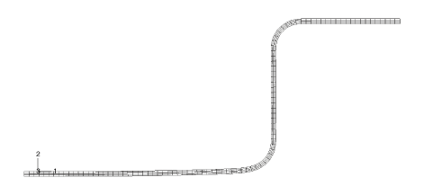
The basic result of this simulation is the deformation of the blank and the plastic strain caused by the forming process. We can plot the deformed model shape and the plastic strain, as described below.
To plot the deformed model shape:
Plot the deformed model shape. You can remove the die and the punch from the display and visualize just the blank.
In the Results Tree, expand the Element sets container underneath the output database file named channel.odb.
From the list of available element sets, select PART-1–1.BLANK. Click mouse button 3, and select Replace from the menu that appears to replace the current display group with the selected elements. Click ![]() , if necessary, to fit the model in the viewport.
, if necessary, to fit the model in the viewport.
The resulting plot is shown in Figure 12–21.
To plot the contours of equivalent plastic strain:
From the main menu bar, select Plot![]() Contours
Contours![]() On Deformed Shape; or click the
On Deformed Shape; or click the ![]() tool from the toolbox to display contours of Mises stress.
tool from the toolbox to display contours of Mises stress.
Open the Contour Plot Options dialog box.
Drag the Contour Intervals slider to change the number of contour intervals to 7.
Click OK to apply these settings.
Select Primary from the list of variable types on the left side of the Field Output toolbar, and select PEEQ from the list of output variables.
PEEQ is an integrated measure of plastic strain. A nonintegrated measure of plastic strain is PEMAG. PEEQ and PEMAG are equal for proportional loading.
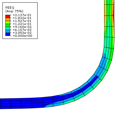
Use the ![]() tool to zoom into any region of interest in the blank, as shown in Figure 12–22.
tool to zoom into any region of interest in the blank, as shown in Figure 12–22.
The maximum plastic strain is approximately 21%. Compare this with the failure strain of the material to determine if the material will tear during the forming process.
History plots of the reaction forces on the blank and punch
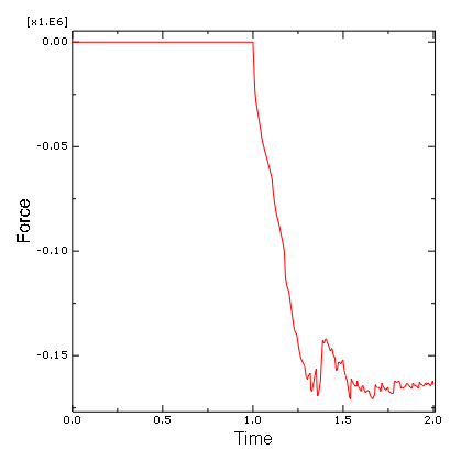
The solid line in Figure 12–23 shows the variation of the reaction force RF2 at the punch's rigid body reference node.
To create a history plot of the reaction force:
In the Results Tree, expand the History Output container. Double-click Reaction force: RF1 PI: PART—1–1 Node xxx in NSET NOUT.
A history plot of the reaction force in the 1-direction appears.
Open the Axis Options dialog box to label the axes.
Switch to the Title tabbed page.
Specify Reaction Force - RF2 as the Y-axis label, and Total Time as the X-axis label.
Click Dismiss to close the dialog box.
The punch force, shown in Figure 12–23, rapidly increases to about 160 kN during Step 2, which runs from a total time of 1.0 to 2.0.
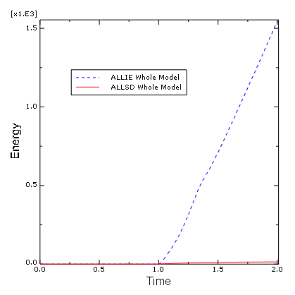
History plot of the stabilization and internal energies
It is important to verify that the presence of contact stabilization does not significantly alter the physics of the problem. One way to assess this requirement is to compare the energy dissipation due to stabilization (ALLSD) against the internal energy of the structure (ALLIE). Ideally the amount of stabilization energy should be a small fraction of the internal energy. Figure 12–24 shows the variation of the stabilization and internal energies. It is clear that the dissipated stabilization energy is indeed small.
Plotting contours on surfaces
Abaqus/Viewer includes a number of features designed specifically for postprocessing contact analyses. The Display Group feature can be used to collect surfaces into display groups, similar to element and node sets.
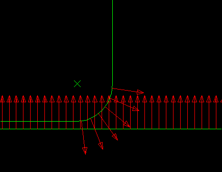
To display contact surface normal vectors:
Plot the undeformed model shape.
In the Results Tree, expand the Surface Sets container. Select the surfaces named BLANK-T and PART—1–1.PUNCH. Click mouse button 3, and select Replace from the menu that appears.
Using the Common Plot Options dialog box, turn on the display of the normal vectors (On surfaces) and set the length of the vector arrows to Short.
Use the ![]() tool, if necessary, to zoom into any region of interest, as shown in Figure 12–25.
tool, if necessary, to zoom into any region of interest, as shown in Figure 12–25.
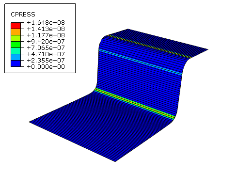
To contour the contact pressure:
Plot the contours of plastic strain again.
From the list of variable types on the left side of the Field Output toolbar, select Primary, if it is not already selected.
From the list of output variables in the center of the toolbar, select CPRESS.
Remove the PART—1–1.PUNCH surface from your display group.
To visualize contours of surface-based variables better in two-dimensional models, you can extrude the plane strain elements to construct the equivalent three-dimensional view. You can sweep axisymmetric elements in a similar fashion.
From the main menu bar, select View![]() ODB Display Options.
ODB Display Options.
The ODB Display Options dialog box appears.
Select the Sweep/Extrude tab to access the Sweep/Extrude options.
In the Extrude region of the dialog box, toggle on Extrude elements; and set the Depth to 0.05 to extrude the model for the purpose of displaying contours.
Click OK to apply these settings.
Rotate the model using the ![]() tool to display the model from a suitable view, such as the one shown in Figure 12–26.
tool to display the model from a suitable view, such as the one shown in Figure 12–26.