You can view a composite layup while you are creating it or after it has been analyzed. Abaqus/CAE provides the following tools for ply-based visualization of a composite layup:
Ply stack plot
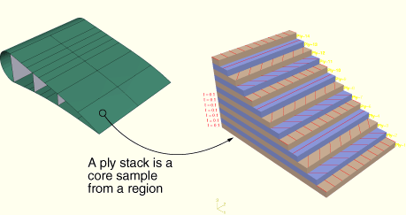
A ply stack plot is a graphical representation of the plies from the selected region of a composite layup or a composite section. Figure 22–9 illustrates a ply stack plot.
The staircase appearance does not indicate ply drop-offs in the layup; it is simply a graphical representation that allows you to see the number of plies in the layup and, for example, the relative thickness of a ply, the material from which it is constructed, and the orientation of its fibers. If your composite layup contains many plies, the ply stack plot can become confusing and hard to interpret. To make the ply stack plot more readable, Abaqus/CAE provides options that allow you to view only a manageable number of plies.The triad in a ply stack plot represents the element orientation system, and it shows the shell normal or stacking direction (the 3-direction) and the 1- and 2-directions for the plies. The fibers are always drawn in the 1–2 plane at an angle with respect to the 1-direction. In solid composite layups the fibers in a ply do not always run parallel to the 1–2 plane (e.g., if the 3-direction of the ply orientation and the element stacking direction are not aligned). In this situation the fibers in the ply stack plot are not a true depiction of the fibers in the layup, but rather a graphical representation of the rotation angles in the layup definition: the angle drawn in the ply stack plot is the rotation angle specified in the ply table measured about the element stacking direction axis. For more information, see “Understanding composite layups and orientations,” Section 22.3.
You can display a ply stack plot in the Property module after you have created a composite layup. You can also display a ply stack plot in the Visualization module after you have analyzed a model with a composite layup. For more information, see Chapter 50, “Viewing a ply stack plot.”
Ply-based results
After you have analyzed a model with a composite layup, you can view a contour plot of results from individual plies of the layup, or you can view an envelope contour plot that looks for maximum or minimum values across all of the plies in the layup.
Results from individual plies
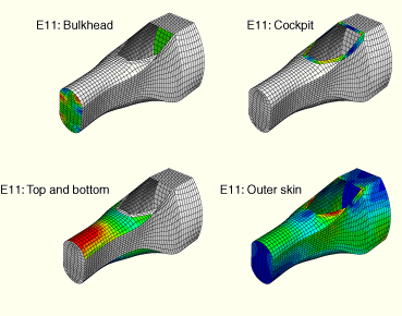
Ply-based results show the data from a selected ply in a composite layup. For a given ply, you can view data from the bottom, middle, or top of the ply, or you can view data from both the top and bottom plies. Figure 22–10 illustrates a contour plot of strain (E11) from selected plies of a composite layup.
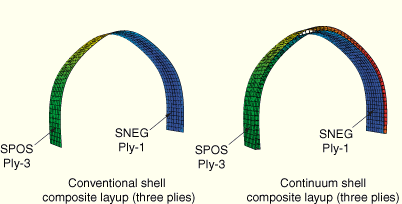
If the same ply name is used in multiple composite layup definitions within a model, viewing data for this ply displays results for all layups in which the ply name appears. To limit the results to a single ply within a single layup, you must first use a display group to limit the display to the individual composite layup (see “Selection methods for creating or editing a display group,” Section 74.2.2), then plot the results for a section point within the desired ply (see “Selecting section point data by ply” in “Selecting section point data,” Section 38.4.8).Contour plots displaying output at both the top and bottom plies of a composite layup vary in appearance depending on the type of layup. In a conventional shell composite layup the two contours appear as a single double-sided shell with different contours on each side. In a continuum shell composite layup or solid composite layup the two contours appear as distinct single-sided contours at each section point location. Figure 22–11 illustrates the difference between contour plots of conventional shell and continuum shell composite layups.
Each layup contains three plies, and each plot is showing the output from the top of the top ply and from the bottom of the bottom ply. Stress (S11) is plotted in both cases. For more information, see “Selecting section point data by category” in “Selecting section point data,” Section 38.4.8.Envelope plots
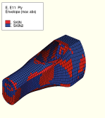
An envelope plot allows you to view a contour plot of the highest or lowest value of a variable in your model, regardless of the ply in which it is occurring. The plies in an envelope plot that correspond with the extreme values are called the critical plies. You can choose the criterion that Abaqus/CAE applies (absolute maximum, maximum, or minimum) and the position in the ply at which Abaqus/CAE checks the value (integration point, centroid, element nodal).
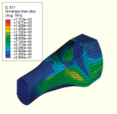
For example, even though your composite layup can include a large number of plies, you can view only the critical plies and determine the highest strain that is occurring in each element of your model. You can decide if you want to reduce the strain in the critical plies by increasing the number of plies in a particular region or by reorienting existing plies. Figure 22–12 shows the value of the strain (E11) in the critical plies of the model.
In addition, you can use the contour plot options to display a quilt contour plot where the color of each element indicates which ply is the critical ply, as shown in Figure 22–13. Using a combination of the plots shown in Figure 22–12 and Figure 22–13, you can determine both the value of the strain in the critical ply and the location of the critical ply in the layup. For more information, see “Selecting the field output to display,” Section 38.4, and “Understanding how contour values are computed,” Section 40.1.1.If you do not create an output request, Abaqus/CAE writes field output data from only the top and bottom of a composite layup, and no data are generated from the other plies. To create an envelope plot that examines all of the plies in your model, you must create a new output request or edit the default output request and specify the composite layup and the plies and section points from which variables will be output.
In many cases, even though you change the position in the ply at which Abaqus/CAE checks the value, the same ply experiences the extreme value, and the contour plot does not change. However, the contour plot might change because the critical ply changed if:
you have a small number of plies, and the results are changing rapidly through the thickness of the ply; or
the material is nonlinear, and its stiffness changes abruptly under some conditions.
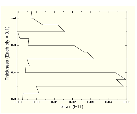
Through thickness X–Y plots
After you have analyzed a composite layup and determined which regions contain the critical plies, you can view the behavior of the plies across the layup with a through thickness X–Y plot. You can create an X–Y data object by reading field output results from the section points in a selected element of a shell region of your model. If you select an element in a composite layup, Abaqus/CAE plots data for each section point in each ply across the entire thickness of the layup. Figure 22–14 illustrates a through thickness plot of the strain in the fiber direction through 13 plies of a composite layup. The strain is discontinuous because the orientation of the fiber changes between plies.
For more information, see “Reading X–Y data through the thickness of a shell,” Section 43.2.3.Color coding
You can use color coding in all of the Abaqus/CAE modules to change the color of individual layups and plies. If you choose to color code by plies, Abaqus/CAE displays only one ply in a region, which by default is the last ply (in alphabetical order). To view a different ply, you can deactivate selected plies. For more information, see “Coloring geometry and mesh elements,” Section 73.4.
Display groups
In the Visualization module you can use display groups to view the elements in only selected layups or plies. For more information, see “Selection methods for creating or editing a display group,” Section 74.2.2.
“Using a composite layup to model a yacht hull,” Section 1.1.24 of the Abaqus Example Problems Manual, illustrates how you can create and analyze a complex three-dimensional composite model and how you can use Abaqus/CAE to view the behavior of individual plies in the layup.